Category: Digital Military History

How have the patterns of American military sacrifice changed throughout the 20th century, and how have said changes influenced our politics in the current year? This question has lingered in my mind for years. While it is a question tangentially related to my dissertation research, it has been a distraction that I cannot shake. I’ve written on this topic for Antiwar.com and on this blog. In both pieces, I argued a thesis that I still hold, that the sectional, economic, and racial disparities in military sacrifice have led to our current political strife.

But what about the past? How did we get here? Assuming that the latter is true, is it a new phenomenon? To answer it, I have, over the last few months, analyzed military fatality data available through the Defense Casualty Analysis System (DCAS) for the Global War on Terror (GWOT), the Vietnam War, as well as the Korean War. Yet, to really flesh this thing out, I needed records for the Second World War…and those are surprisingly difficult to obtain, at least in a transcribed form.

So I decided to do it myself and hand-jammed the county tabulations in the “WWII Army and Army Air Force Casualties” records currently available in pdf form from the National Archives. The records contain 3,123 county figures for all 48 states plus Washington, D.C., and total up to 307,757 U.S. Army and U.S. Army Air Forces killed and missing in action. I should note that the records also contain the names and geographic tabulations of those who hailed from America’s various territories (including Hawaii and Alaska).

These records do not contain figures for those who served within the Department of the Navy, which includes sailors, marines, and coastguardsmen. While the Navy records do list individuals and their street addresses, they do not offer county-level tabulations. I have, however, digitized the Navy Department’s state records and posted a CSV file with them and the Department of the Army figures. The said file is available on my GitHub.

Attempting a long-term analysis of county-level military fatalities without data from the Navy is, in the parlance of our times, problematic. The NARA records record that 66,370 sailors, marines, and coastguardmen were killed in the war. But there’s no way that I can, as a single person, transcribe every name and then geocode every address.

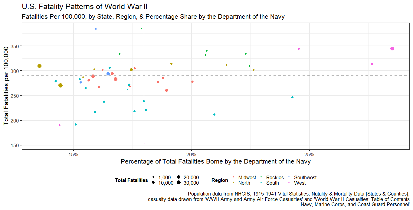
Spoiler alert: we’re still going to proceed, but before doing so, I’d like to pause and note that according to these datasets, 17.9% of American lives were lost during the war came from those who served within the Department of the Navy. They were not spread out evenly as 19 states endured slanted naval losses above the national average, including some highly populated states like California (graphic 1).

Even with incomplete records, that is, only those county-level statistics from the Department of the Army, I think we can still proceed with our inquiry. To make sense of the fatality records, I analyzed them against demographic data from the U.S. Census and the “1915-1941 Vital Statistics: Natality & Mortality Data [States & Counties]” made available through the National Historical Geographic Information System.¹

Generating per capita statistics for the Department of the Army losses during the Second World War yields the following results (see interactive table below).

The table lists the county, state, and number of Army fatalities per 100k losses and the county’s percentage difference from the national per 100k (233.455). If you sort the records by the number of losses, unsurprisingly, the most populous county in 1940, Cook County, which contains Chicago, is at the top of the list. But, what is different from subsequent wars (to varying degrees, as we shall see) is that these highly populated counties all meet, exceed, or at the least come close to the national per 100k.

County	State	Number	Population in 1940	Fatalities Per 100k	Difference from National Per 100k
Autauga	Alabama	32	20977	152.5	65.3%
Baldwin	Alabama	44	32324	136.1	58.3%
Barbour	Alabama	36	32722	110.0	47.1%
Bibb	Alabama	39	20155	193.5	82.9%
Blount	Alabama	44	29490	149.2	63.9%
Bullock	Alabama	20	19810	101.0	43.2%
Butler	Alabama	58	32447	178.8	76.6%
Calhoun	Alabama	169	63319	266.9	114.3%
Chambers	Alabama	58	42146	137.6	58.9%
Cherokee	Alabama	29	19928	145.5	62.3%
Chilton	Alabama	49	27955	175.3	75.1%
Choctaw	Alabama	31	20195	153.5	65.8%
Clarke	Alabama	38	27636	137.5	58.9%
Clay	Alabama	27	16907	159.7	68.4%
Cleburne	Alabama	22	13629	161.4	69.1%
Coffee	Alabama	52	31987	162.6	69.6%
Colbert	Alabama	74	34093	217.1	93.0%
Conecuh	Alabama	27	25489	105.9	45.4%
Coosa	Alabama	30	13460	222.9	95.5%
Covington	Alabama	88	42417	207.5	88.9%
Crenshaw	Alabama	36	23631	152.3	65.3%
Cullman	Alabama	116	47343	245.0	105.0%
Dale	Alabama	35	22685	154.3	66.1%
Dallas	Alabama	71	55245	128.5	55.1%
De Kalb	Alabama	103	43075	239.1	102.4%
Elmore	Alabama	69	34546	199.7	85.6%
Escambia	Alabama	60	30671	195.6	83.8%
Etowah	Alabama	143	72580	197.0	84.4%
Fayette	Alabama	52	21651	240.2	102.9%
Franklin	Alabama	69	27552	250.4	107.3%
Geneva	Alabama	55	29172	188.5	80.8%
Greene	Alabama	10	19185	52.1	22.3%
Hale	Alabama	26	25533	101.8	43.6%
Henry	Alabama	23	21912	105.0	45.0%
Houston	Alabama	73	45665	159.9	68.5%
Jackson	Alabama	106	41802	253.6	108.6%
Jefferson	Alabama	874	459930	190.0	81.4%
Lamar	Alabama	39	19708	197.9	84.8%
Lauderdale	Alabama	90	46230	194.7	83.4%
Lawrence	Alabama	43	27880	154.2	66.1%
Lee	Alabama	62	36455	170.1	72.9%
Limestone	Alabama	59	35642	165.5	70.9%
Lowndes	Alabama	15	22661	66.2	28.4%
Macon	Alabama	28	27654	101.3	43.4%
Madison	Alabama	132	66317	199.0	85.3%
Marengo	Alabama	29	35736	81.2	34.8%
Marion	Alabama	74	28776	257.2	110.2%
Marshall	Alabama	102	42395	240.6	103.1%
Mobile	Alabama	249	141974	175.4	75.1%
Monroe	Alabama	24	29465	81.5	34.9%
Montgomery	Alabama	209	114420	182.7	78.2%
Morgan	Alabama	110	48148	228.5	97.9%
Perry	Alabama	21	26610	78.9	33.8%
Pickens	Alabama	40	27671	144.6	61.9%
Pike	Alabama	36	32493	110.8	47.5%
Randolph	Alabama	54	25516	211.6	90.7%
Russell	Alabama	51	35775	142.6	61.1%
Shelby	Alabama	41	28962	141.6	60.6%
St Clair	Alabama	63	27336	230.5	98.7%
Sumter	Alabama	21	27321	76.9	32.9%
Talladega	Alabama	132	51832	254.7	109.1%
Tallapoosa	Alabama	59	35270	167.3	71.7%
Tuscaloosa	Alabama	149	76036	196.0	83.9%
Walker	Alabama	150	64201	233.6	100.1%
Washington	Alabama	31	16188	191.5	82.0%
Wilcox	Alabama	34	26279	129.4	55.4%
Winston	Alabama	42	18746	224.0	96.0%
Arkansas	Arkansas	52	24437	212.8	91.1%
Ashley	Arkansas	52	26785	194.1	83.2%
Baxter	Arkansas	30	10281	291.8	125.0%
Benton	Arkansas	99	36148	273.9	117.3%
Boone	Arkansas	47	15860	296.3	126.9%
Bradley	Arkansas	39	18097	215.5	92.3%
Calhoun	Arkansas	29	9636	301.0	128.9%
Carroll	Arkansas	36	14737	244.3	104.6%
Chicot	Arkansas	32	27452	116.6	49.9%
Clark	Arkansas	49	24402	200.8	86.0%
Clay	Arkansas	65	28386	229.0	98.1%
Cleburne	Arkansas	26	13134	198.0	84.8%
Cleveland	Arkansas	22	12570	175.0	75.0%
Columbia	Arkansas	48	29822	161.0	68.9%
Conway	Arkansas	32	21536	148.6	63.6%
Craighead	Arkansas	100	47200	211.9	90.8%
Crawford	Arkansas	62	23920	259.2	111.0%
Crittenden	Arkansas	25	42473	58.9	25.2%
Cross	Arkansas	57	26046	218.8	93.7%
Dallas	Arkansas	22	14471	152.0	65.1%
Desha	Arkansas	46	27160	169.4	72.5%
Drew	Arkansas	30	19831	151.3	64.8%
Faulkner	Arkansas	62	25880	239.6	102.6%
Franklin	Arkansas	36	15683	229.5	98.3%
Fulton	Arkansas	27	10253	263.3	112.8%
Garland	Arkansas	95	41664	228.0	97.7%
Grant	Arkansas	24	10477	229.1	98.1%
Greene	Arkansas	50	30204	165.5	70.9%
Hempstead	Arkansas	52	32770	158.7	68.0%
Hot Spring	Arkansas	55	18916	290.8	124.5%
Howard	Arkansas	35	16621	210.6	90.2%
Independence	Arkansas	62	25643	241.8	103.6%
Izard	Arkansas	34	12834	264.9	113.5%
Jackson	Arkansas	50	26427	189.2	81.0%
Jefferson	Arkansas	86	65101	132.1	56.6%
Johnson	Arkansas	36	18795	191.5	82.0%
Lafayette	Arkansas	19	16851	112.8	48.3%
Lawrence	Arkansas	47	22651	207.5	88.9%
Lee	Arkansas	24	26810	89.5	38.3%
Lincoln	Arkansas	28	19709	142.1	60.9%
Little River	Arkansas	31	15932	194.6	83.3%
Logan	Arkansas	60	25967	231.1	99.0%
Lonoke	Arkansas	55	29802	184.6	79.1%
Madison	Arkansas	29	14531	199.6	85.5%
Marion	Arkansas	17	9464	179.6	76.9%
Miller	Arkansas	55	31874	172.6	73.9%
Mississippi	Arkansas	115	80217	143.4	61.4%
Monroe	Arkansas	33	21133	156.2	66.9%
Montgomery	Arkansas	22	8876	247.9	106.2%
Nevada	Arkansas	43	19869	216.4	92.7%
Newton	Arkansas	23	10881	211.4	90.5%
Ouachita	Arkansas	52	31151	166.9	71.5%
Perry	Arkansas	17	8392	202.6	86.8%
Phillips	Arkansas	53	45970	115.3	49.4%
Pike	Arkansas	29	11786	246.1	105.4%
Poinsett	Arkansas	85	37670	225.6	96.7%
Polk	Arkansas	47	15832	296.9	127.2%
Pope	Arkansas	35	25682	136.3	58.4%
Prairie	Arkansas	34	15304	222.2	95.2%
Pulaski	Arkansas	327	156085	209.5	89.7%
Randolph	Arkansas	30	18319	163.8	70.1%
Saline	Arkansas	38	19163	198.3	84.9%
Scott	Arkansas	26	13300	195.5	83.7%
Searcy	Arkansas	24	11942	201.0	86.1%
Sebastian	Arkansas	154	62809	245.2	105.0%
Sevier	Arkansas	34	15248	223.0	95.5%
Sharp	Arkansas	27	11497	234.8	100.6%
St Francis	Arkansas	41	36043	113.8	48.7%
St.one	Arkansas	14	8603	162.7	69.7%
Union	Arkansas	94	50461	186.3	79.8%
Van Buren	Arkansas	36	12518	287.6	123.2%
Washington	Arkansas	105	41114	255.4	109.4%
White	Arkansas	76	37176	204.4	87.6%
Woodruff	Arkansas	32	22133	144.6	61.9%
Yell	Arkansas	48	20970	228.9	98.0%
Apache	Arizona	51	24095	211.7	90.7%
Cochise	Arizona	111	34627	320.6	137.3%
Coconino	Arizona	49	18770	261.1	111.8%
Gila	Arizona	87	23867	364.5	156.1%
Graham	Arizona	49	12113	404.5	173.3%
Greenlee	Arizona	31	8698	356.4	152.7%
Maricopa	Arizona	514	186193	276.1	118.2%
Mohave	Arizona	22	8591	256.1	109.7%
Navajo	Arizona	64	25309	252.9	108.3%
Pima	Arizona	239	72838	328.1	140.6%
Pinal	Arizona	115	28841	398.7	170.8%
Santa Cruz	Arizona	43	9482	453.5	194.3%
Yavapai	Arizona	80	26511	301.8	129.3%
Yuma	Arizona	80	19326	414.0	177.3%
Alameda	California	1266	513011	246.8	105.7%
Alpine	California	1	323	309.6	132.6%
Amador	California	22	8973	245.2	105.0%
Butte	California	107	42840	249.8	107.0%
Calaveras	California	21	8221	255.4	109.4%
Colusa	California	25	9788	255.4	109.4%
Contra Costa	California	320	100450	318.6	136.5%
Del Norte	California	7	4745	147.5	63.2%
El Dorado	California	27	13229	204.1	87.4%
Fresno	California	511	178565	286.2	122.6%
Glenn	California	32	12195	262.4	112.4%
Humboldt	California	114	45812	248.8	106.6%
Imperial	California	107	59740	179.1	76.7%
Inyo	California	28	7625	367.2	157.3%
Kern	California	340	135124	251.6	107.8%
Kings	California	104	35168	295.7	126.7%
Lake	California	26	8069	322.2	138.0%
Lassen	California	49	14479	338.4	145.0%
Los Angeles	California	6674	2785643	239.6	102.6%
Madera	California	79	23314	338.9	145.1%
Marin	California	103	52907	194.7	83.4%
Mariposa	California	6	5605	107.0	45.9%
Mendocino	California	54	27864	193.8	83.0%
Merced	California	103	46988	219.2	93.9%
Modoc	California	23	8713	264.0	113.1%
Mono	California	11	2299	478.5	205.0%
Monterey	California	240	73032	328.6	140.8%
Napa	California	57	28503	200.0	85.7%
Nevada	California	42	19283	217.8	93.3%
Orange	California	334	130760	255.4	109.4%
Placer	California	75	28108	266.8	114.3%
Plumas	California	49	11548	424.3	181.8%
Riverside	California	314	105524	297.6	127.5%
Sacramento	California	441	170333	258.9	110.9%
San Benito	California	36	11392	316.0	135.4%
San Bernardino	California	441	161108	273.7	117.3%
San Diego	California	775	289348	267.8	114.7%
San Francisco	California	1365	634536	215.1	92.1%
San Joaquin	California	283	134207	210.9	90.3%
San Luis Obispo	California	89	33246	267.7	114.7%
San Mateo	California	220	111782	196.8	84.3%
Santa Barbara	California	153	70555	216.9	92.9%
Santa Clara	California	441	174949	252.1	108.0%
Santa Cruz	California	88	45057	195.3	83.7%
Shasta	California	69	28800	239.6	102.6%
Sierra	California	12	3025	396.7	169.9%
Siskiyou	California	72	28598	251.8	107.8%
Solano	California	150	49118	305.4	130.8%
Sonoma	California	165	69052	239.0	102.4%
St.anislaus	California	178	74866	237.8	101.8%
Sutter	California	61	18680	326.6	139.9%
Tehama	California	17	14316	118.7	50.9%
Trinity	California	9	3970	226.7	97.1%
Tulare	California	246	107152	229.6	98.3%
Tuolumne	California	26	10887	238.8	102.3%
Ventura	California	216	69685	310.0	132.8%
Yolo	California	72	27243	264.3	113.2%
Yuba	California	45	17034	264.2	113.2%
Adams	Colorado	42	22481	186.8	80.0%
Alamosa	Colorado	34	10484	324.3	138.9%
Arapahoe	Colorado	64	32150	199.1	85.3%
Archuleta	Colorado	17	3806	446.7	191.3%
Baca	Colorado	14	6207	225.6	96.6%
Bent	Colorado	25	9653	259.0	110.9%
Boulder	Colorado	88	37438	235.1	100.7%
Chaffee	Colorado	18	8109	222.0	95.1%
Cheyenne	Colorado	9	2964	303.6	130.1%
Clear Creek	Colorado	9	3784	237.8	101.9%
Conejos	Colorado	31	11648	266.1	114.0%
Costilla	Colorado	11	7533	146.0	62.5%
Crowley	Colorado	22	5398	407.6	174.6%
Custer	Colorado	7	2270	308.4	132.1%
Delta	Colorado	44	16470	267.2	114.4%
Denver	Colorado	786	322412	243.8	104.4%
Dolores	Colorado	1	1958	51.1	21.9%
Douglas	Colorado	7	3496	200.2	85.8%
Eagle	Colorado	7	5361	130.6	55.9%
Elbert	Colorado	3	5460	54.9	23.5%
El Paso	Colorado	141	54025	261.0	111.8%
Fremont	Colorado	53	19742	268.5	115.0%
Garfield	Colorado	29	10560	274.6	117.6%
Gilpin	Colorado	1	1625	61.5	26.4%
Grand	Colorado	14	3587	390.3	167.2%
Gunnison	Colorado	16	6192	258.4	110.7%
Hinsdale	Colorado	2	349	573.1	245.5%
Huerfano	Colorado	42	16088	261.1	111.8%
Jackson	Colorado	6	1798	333.7	142.9%
Jefferson	Colorado	57	30725	185.5	79.5%
Kiowa	Colorado	15	2793	537.1	230.0%
Kit Carson	Colorado	16	7512	213.0	91.2%
Lake	Colorado	19	6883	276.0	118.2%
La Plata	Colorado	39	15494	251.7	107.8%
Larimer	Colorado	77	35539	216.7	92.8%
Las Animas	Colorado	81	32369	250.2	107.2%
Lincoln	Colorado	17	5882	289.0	123.8%
Logan	Colorado	39	18370	212.3	90.9%
Mesa	Colorado	73	33791	216.0	92.5%
Mineral	Colorado	1	975	102.6	43.9%
Moffat	Colorado	15	5086	294.9	126.3%
Montezuma	Colorado	20	10463	191.1	81.9%
Montrose	Colorado	45	15418	291.9	125.0%
Morgan	Colorado	50	17214	290.5	124.4%
Otero	Colorado	39	23571	165.5	70.9%
Ouray	Colorado	4	2089	191.5	82.0%
Park	Colorado	7	3272	213.9	91.6%
Phillips	Colorado	18	4948	363.8	155.8%
Pitkin	Colorado	2	1836	108.9	46.7%
Prowers	Colorado	44	12304	357.6	153.2%
Pueblo	Colorado	151	68870	219.3	93.9%
Rio Blanco	Colorado	14	2943	475.7	203.8%
Rio Grande	Colorado	30	12404	241.9	103.6%
Routt	Colorado	25	10525	237.5	101.7%
Saguache	Colorado	14	6173	226.8	97.1%
San Juan	Colorado	3	1439	208.5	89.3%
San Miguel	Colorado	8	3664	218.3	93.5%
Sedgwick	Colorado	9	5294	170.0	72.8%
Summit	Colorado	2	1754	114.0	48.8%
Teller	Colorado	15	6463	232.1	99.4%
Washington	Colorado	11	8336	132.0	56.5%
Weld	Colorado	136	63747	213.3	91.4%
Yuma	Colorado	30	12102	247.9	106.2%
Fairfield	Connecticut	1097	418384	262.2	112.3%
Hartford	Connecticut	1238	450189	275.0	117.8%
Litchfield	Connecticut	232	87041	266.5	114.2%
Middlesex	Connecticut	136	55999	242.9	104.0%
New Haven	Connecticut	1143	484316	236.0	101.1%
New London	Connecticut	250	125224	199.6	85.5%
Tolland	Connecticut	66	31866	207.1	88.7%
Windham	Connecticut	147	56223	261.5	112.0%
District Of Columbia	District of Columbia	3029	663091	456.8	195.7%
Kent	Delaware	59	34441	171.3	73.4%
New Castle	Delaware	392	179562	218.3	93.5%
Sussex	Delaware	91	52502	173.3	74.2%
Alachua	Florida	59	38607	152.8	65.5%
Baker	Florida	18	6510	276.5	118.4%
Bay	Florida	56	20686	270.7	116.0%
Bradford	Florida	17	8717	195.0	83.5%
Brevard	Florida	26	16142	161.1	69.0%
Broward	Florida	50	39794	125.6	53.8%
Calhoun	Florida	24	8218	292.0	125.1%
Charlotte	Florida	8	3663	218.4	93.6%
Citrus	Florida	16	5846	273.7	117.2%
Clay	Florida	13	6468	201.0	86.1%
Collier	Florida	8	5102	156.8	67.2%
Columbia	Florida	27	16859	160.2	68.6%
De Soto	Florida	13	7792	166.8	71.5%
Dixie	Florida	10	7018	142.5	61.0%
Duval	Florida	392	210143	186.5	79.9%
Escambia	Florida	124	74667	166.1	71.1%
Flagler	Florida	5	3008	166.2	71.2%
Franklin	Florida	11	5991	183.6	78.6%
Gadsden	Florida	43	31450	136.7	58.6%
Gilchrist	Florida	9	4250	211.8	90.7%
Glades	Florida	6	2745	218.6	93.6%
Gulf	Florida	17	6951	244.6	104.8%
Hamilton	Florida	13	9778	133.0	56.9%
Hardee	Florida	25	10158	246.1	105.4%
Hendry	Florida	16	5237	305.5	130.9%
Hernando	Florida	15	5641	265.9	113.9%
Highlands	Florida	28	9246	302.8	129.7%
Hillsborough	Florida	363	180148	201.5	86.3%
Holmes	Florida	35	15447	226.6	97.1%
Indian River	Florida	16	8957	178.6	76.5%
Jackson	Florida	54	34428	156.8	67.2%
Jefferson	Florida	9	12032	74.8	32.0%
Lafayette	Florida	6	4405	136.2	58.3%
Lake	Florida	53	27255	194.5	83.3%
Lee	Florida	43	17488	245.9	105.3%
Leon	Florida	56	31646	177.0	75.8%
Levy	Florida	23	12550	183.3	78.5%
Liberty	Florida	10	3752	266.5	114.2%
Madison	Florida	19	16190	117.4	50.3%
Manatee	Florida	46	26098	176.3	75.5%
Marion	Florida	44	31243	140.8	60.3%
Martin	Florida	7	6295	111.2	47.6%
Dade	Florida	503	267739	187.9	80.5%
Monroe	Florida	30	14078	213.1	91.3%
Nassau	Florida	15	10826	138.6	59.3%
Okaloosa	Florida	34	12900	263.6	112.9%
Okeechobee	Florida	7	3000	233.3	99.9%
Orange	Florida	173	70074	246.9	105.8%
Osceola	Florida	14	10119	138.4	59.3%
Palm Beach	Florida	122	79989	152.5	65.3%
Pasco	Florida	29	13981	207.4	88.8%
Pinellas	Florida	138	91852	150.2	64.4%
Polk	Florida	200	86665	230.8	98.9%
Putnam	Florida	25	18698	133.7	57.3%
Santa Rosa	Florida	28	16085	174.1	74.6%
Sarasota	Florida	33	16106	204.9	87.8%
Seminole	Florida	37	22304	165.9	71.1%
St Johns	Florida	41	20012	204.9	87.8%
St Lucie	Florida	20	11871	168.5	72.2%
Sumter	Florida	19	11041	172.1	73.7%
Suwannee	Florida	29	17073	169.9	72.8%
Taylor	Florida	16	11565	138.3	59.3%
Union	Florida	9	7094	126.9	54.3%
Volusia	Florida	87	53710	162.0	69.4%
Wakulla	Florida	8	5463	146.4	62.7%
Walton	Florida	31	14246	217.6	93.2%
Washington	Florida	25	12302	203.2	87.0%
Appling	Georgia	33	14497	227.6	97.5%
Atkinson	Georgia	12	7093	169.2	72.5%
Bacon	Georgia	15	8096	185.3	79.4%
Baker	Georgia	5	7344	68.1	29.2%
Baldwin	Georgia	29	24190	119.9	51.4%
Banks	Georgia	11	8733	126.0	54.0%
Barrow	Georgia	40	13064	306.2	131.2%
Bartow	Georgia	47	25283	185.9	79.6%
Ben Hill	Georgia	22	14523	151.5	64.9%
Berrien	Georgia	18	15370	117.1	50.2%
Bibb	Georgia	160	83783	191.0	81.8%
Bleckley	Georgia	22	9655	227.9	97.6%
Brantley	Georgia	17	6871	247.4	106.0%
Brooks	Georgia	23	20497	112.2	48.1%
Bryan	Georgia	12	6288	190.8	81.7%
Bulloch	Georgia	33	26010	126.9	54.3%
Burke	Georgia	24	26520	90.5	38.8%
Butts	Georgia	19	9182	206.9	88.6%
Calhoun	Georgia	16	10438	153.3	65.7%
Camden	Georgia	7	5910	118.4	50.7%
Candler	Georgia	11	9103	120.8	51.8%
Carroll	Georgia	78	34156	228.4	97.8%
Catoosa	Georgia	19	12199	155.8	66.7%
Charlton	Georgia	17	5256	323.4	138.5%
Chatham	Georgia	223	117970	189.0	81.0%
Chattahoochee	Georgia	12	15138	79.3	34.0%
Chattooga	Georgia	43	18532	232.0	99.4%
Cherokee	Georgia	42	20126	208.7	89.4%
Clarke	Georgia	59	28398	207.8	89.0%
Clay	Georgia	9	7064	127.4	54.6%
Clayton	Georgia	25	11655	214.5	91.9%
Clinch	Georgia	7	6437	108.7	46.6%
Cobb	Georgia	70	38272	182.9	78.3%
Coffee	Georgia	42	21541	195.0	83.5%
Colquitt	Georgia	58	33012	175.7	75.3%
Columbia	Georgia	12	9433	127.2	54.5%
Cook	Georgia	30	11919	251.7	107.8%
Coweta	Georgia	42	26972	155.7	66.7%
Crawford	Georgia	12	7128	168.4	72.1%
Crisp	Georgia	24	17540	136.8	58.6%
Dade	Georgia	13	5894	220.6	94.5%
Dawson	Georgia	9	4479	200.9	86.1%
Decatur	Georgia	49	22234	220.4	94.4%
Dekalb	Georgia	120	86942	138.0	59.1%
Dodge	Georgia	33	21022	157.0	67.2%
Dooly	Georgia	25	16886	148.1	63.4%
Dougherty	Georgia	55	28565	192.5	82.5%
Douglas	Georgia	15	10053	149.2	63.9%
Early	Georgia	14	18679	75.0	32.1%
Echols	Georgia	4	2964	135.0	57.8%
Effingham	Georgia	13	9646	134.8	57.7%
Elbert	Georgia	31	19618	158.0	67.7%
Emanuel	Georgia	32	23517	136.1	58.3%
Evans	Georgia	10	7401	135.1	57.9%
Fannin	Georgia	30	14752	203.4	87.1%
Fayette	Georgia	14	8170	171.4	73.4%
Floyd	Georgia	115	56141	204.8	87.7%
Forsyth	Georgia	13	11322	114.8	49.2%
Franklin	Georgia	24	15612	153.7	65.8%
Fulton	Georgia	883	392886	224.7	96.3%
Gilmer	Georgia	26	9001	288.9	123.7%
Glascock	Georgia	10	4547	219.9	94.2%
Glynn	Georgia	60	21920	273.7	117.2%
Gordon	Georgia	43	18445	233.1	99.9%
Grady	Georgia	33	19654	167.9	71.9%
Greene	Georgia	27	13709	197.0	84.4%
Gwinnett	Georgia	57	29087	196.0	83.9%
Habersham	Georgia	30	14771	203.1	87.0%
Hall	Georgia	99	34822	284.3	121.8%
Hancock	Georgia	18	12764	141.0	60.4%
Haralson	Georgia	28	14377	194.8	83.4%
Harris	Georgia	16	11428	140.0	60.0%
Hart	Georgia	26	15512	167.6	71.8%
Heard	Georgia	12	8610	139.4	59.7%
Henry	Georgia	20	15119	132.3	56.7%
Houston	Georgia	12	11303	106.2	45.5%
Irwin	Georgia	10	12936	77.3	33.1%
Jackson	Georgia	48	20089	238.9	102.3%
Jasper	Georgia	19	8772	216.6	92.8%
Jeff Davis	Georgia	13	8841	147.0	63.0%
Jefferson	Georgia	32	20040	159.7	68.4%
Jenkins	Georgia	16	11843	135.1	57.9%
Johnson	Georgia	18	12953	139.0	59.5%
Jones	Georgia	10	8331	120.0	51.4%
Lamar	Georgia	23	10091	227.9	97.6%
Lanier	Georgia	13	5632	230.8	98.9%
Laurens	Georgia	76	33606	226.2	96.9%
Lee	Georgia	8	7837	102.1	43.7%
Liberty	Georgia	12	8595	139.6	59.8%
Lincoln	Georgia	7	7042	99.4	42.6%
Long	Georgia	6	4086	146.8	62.9%
Lowndes	Georgia	50	31860	156.9	67.2%
Lumpkin	Georgia	14	6223	225.0	96.4%
Macon	Georgia	44	15947	275.9	118.2%
Madison	Georgia	32	13431	238.3	102.1%
Marion	Georgia	5	6954	71.9	30.8%
Mcduffie	Georgia	31	10878	285.0	122.1%
Meriwether	Georgia	36	22055	163.2	69.9%
Miller	Georgia	12	9998	120.0	51.4%
Mitchell	Georgia	27	23261	116.1	49.7%
Monroe	Georgia	11	10749	102.3	43.8%
Montgomery	Georgia	7	9668	72.4	31.0%
Morgan	Georgia	20	12713	157.3	67.4%
Murray	Georgia	23	11137	206.5	88.5%
Muscogee	Georgia	207	75494	274.2	117.5%
Newton	Georgia	36	18576	193.8	83.0%
Oconee	Georgia	16	7576	211.2	90.5%
Oglethorpe	Georgia	6	12430	48.3	20.7%
Paulding	Georgia	21	12832	163.7	70.1%
Peach	Georgia	20	10378	192.7	82.5%
Pickens	Georgia	13	9136	142.3	61.0%
Pierce	Georgia	24	11800	203.4	87.1%
Pike	Georgia	18	10375	173.5	74.3%
Polk	Georgia	64	28467	224.8	96.3%
Pulaski	Georgia	12	9829	122.1	52.3%
Putnam	Georgia	12	8514	140.9	60.4%
Quitman	Georgia	8	3435	232.9	99.8%
Rabun	Georgia	20	7821	255.7	109.5%
Randolph	Georgia	12	16609	72.2	30.9%
Richmond	Georgia	138	81863	168.6	72.2%
Rockdale	Georgia	14	7724	181.3	77.6%
Schley	Georgia	8	5033	159.0	68.1%
Screven	Georgia	31	20353	152.3	65.2%
Seminole	Georgia	13	8492	153.1	65.6%
Spalding	Georgia	62	28427	218.1	93.4%
St.ephens	Georgia	38	12972	292.9	125.5%
St.ewart	Georgia	10	10603	94.3	40.4%
Sumter	Georgia	35	24502	142.8	61.2%
Talbot	Georgia	5	8141	61.4	26.3%
Taliaferro	Georgia	4	6278	63.7	27.3%
Tattnall	Georgia	26	16243	160.1	68.6%
Taylor	Georgia	17	10768	157.9	67.6%
Telfair	Georgia	26	15145	171.7	73.5%
Terrell	Georgia	24	16675	143.9	61.7%
Thomas	Georgia	49	31289	156.6	67.1%
Tift	Georgia	34	18599	182.8	78.3%
Toombs	Georgia	31	16952	182.9	78.3%
Towns	Georgia	13	4925	264.0	113.1%
Treutlen	Georgia	9	7632	117.9	50.5%
Troup	Georgia	84	43879	191.4	82.0%
Turner	Georgia	16	10846	147.5	63.2%
Twiggs	Georgia	5	9117	54.8	23.5%
Union	Georgia	14	7680	182.3	78.1%
Upson	Georgia	45	25064	179.5	76.9%
Walker	Georgia	83	31024	267.5	114.6%
Walton	Georgia	31	20777	149.2	63.9%
Ware	Georgia	58	27929	207.7	89.0%
Warren	Georgia	13	10236	127.0	54.4%
Washington	Georgia	34	24230	140.3	60.1%
Wayne	Georgia	21	13122	160.0	68.6%
Webster	Georgia	1	4726	21.2	9.1%
Wheeler	Georgia	17	8535	199.2	85.3%
White	Georgia	12	6417	187.0	80.1%
Whitfield	Georgia	56	26105	214.5	91.9%
Wilcox	Georgia	27	12755	211.7	90.7%
Wilkes	Georgia	9	15084	59.7	25.6%
Wilkinson	Georgia	12	11025	108.8	46.6%
Worth	Georgia	19	21374	88.9	38.1%
Adair	Iowa	34	13196	257.7	110.4%
Adams	Iowa	27	10156	265.9	113.9%
Allamakee	Iowa	30	17184	174.6	74.8%
Appanoose	Iowa	65	24245	268.1	114.8%
Audubon	Iowa	31	11790	262.9	112.6%
Benton	Iowa	54	22879	236.0	101.1%
Black Hawk	Iowa	201	79946	251.4	107.7%
Boone	Iowa	66	29782	221.6	94.9%
Bremer	Iowa	29	17932	161.7	69.3%
Buchanan	Iowa	33	20991	157.2	67.3%
Buena Vista	Iowa	35	19838	176.4	75.6%
Butler	Iowa	38	17986	211.3	90.5%
Calhoun	Iowa	43	17584	244.5	104.7%
Carroll	Iowa	50	22770	219.6	94.1%
Cass	Iowa	47	18647	252.1	108.0%
Cedar	Iowa	35	16884	207.3	88.8%
Cerro Gordo	Iowa	112	43845	255.4	109.4%
Cherokee	Iowa	37	19258	192.1	82.3%
Chickasaw	Iowa	30	15227	197.0	84.4%
Clarke	Iowa	20	10233	195.4	83.7%
Clay	Iowa	30	17762	168.9	72.3%
Clayton	Iowa	36	24334	147.9	63.4%
Clinton	Iowa	101	44722	225.8	96.7%
Crawford	Iowa	56	20538	272.7	116.8%
Dallas	Iowa	55	24649	223.1	95.6%
Davis	Iowa	27	11136	242.5	103.9%
Decatur	Iowa	47	14012	335.4	143.7%
Delaware	Iowa	35	18487	189.3	81.1%
Des Moines	Iowa	105	36804	285.3	122.2%
Dickinson	Iowa	23	12185	188.8	80.9%
Dubuque	Iowa	162	63768	254.0	108.8%
Emmet	Iowa	40	13406	298.4	127.8%
Fayette	Iowa	55	29151	188.7	80.8%
Floyd	Iowa	49	20169	242.9	104.1%
Franklin	Iowa	24	16379	146.5	62.8%
Fremont	Iowa	46	14645	314.1	134.5%
Greene	Iowa	46	16599	277.1	118.7%
Grundy	Iowa	34	13518	251.5	107.7%
Guthrie	Iowa	38	17210	220.8	94.6%
Hamilton	Iowa	46	19922	230.9	98.9%
Hancock	Iowa	26	15402	168.8	72.3%
Hardin	Iowa	32	22530	142.0	60.8%
Harrison	Iowa	45	22767	197.7	84.7%
Henry	Iowa	39	17994	216.7	92.8%
Howard	Iowa	29	13531	214.3	91.8%
Humboldt	Iowa	32	13459	237.8	101.8%
Ida	Iowa	23	11047	208.2	89.2%
Iowa	Iowa	33	17016	193.9	83.1%
Jackson	Iowa	27	19181	140.8	60.3%
Jasper	Iowa	64	31496	203.2	87.0%
Jefferson	Iowa	43	15762	272.8	116.9%
Johnson	Iowa	75	33191	226.0	96.8%
Jones	Iowa	33	19950	165.4	70.9%
Keokuk	Iowa	43	18406	233.6	100.1%
Kossuth	Iowa	69	26630	259.1	111.0%
Lee	Iowa	98	41074	238.6	102.2%
Linn	Iowa	213	89142	238.9	102.4%
Louisa	Iowa	25	11384	219.6	94.1%
Lucas	Iowa	21	14571	144.1	61.7%
Lyon	Iowa	27	15374	175.6	75.2%
Madison	Iowa	23	14525	158.3	67.8%
Mahaska	Iowa	54	26485	203.9	87.3%
Marion	Iowa	35	27019	129.5	55.5%
Marshall	Iowa	52	35406	146.9	62.9%
Mills	Iowa	31	15064	205.8	88.1%
Mitchell	Iowa	32	14121	226.6	97.1%
Monona	Iowa	41	18238	224.8	96.3%
Monroe	Iowa	32	14553	219.9	94.2%
Montgomery	Iowa	46	15697	293.0	125.5%
Muscatine	Iowa	64	31296	204.5	87.6%
O'brien	Iowa	42	19293	217.7	93.2%
Osceola	Iowa	13	10607	122.6	52.5%
Page	Iowa	56	24887	225.0	96.4%
Palo Alto	Iowa	44	16170	272.1	116.6%
Plymouth	Iowa	54	23502	229.8	98.4%
Pocahontas	Iowa	33	16266	202.9	86.9%
Polk	Iowa	450	195835	229.8	98.4%
Pottawattamie	Iowa	152	66756	227.7	97.5%
Poweshiek	Iowa	41	18758	218.6	93.6%
Ringgold	Iowa	28	11137	251.4	107.7%
Sac	Iowa	28	17639	158.7	68.0%
Scott	Iowa	168	84748	198.2	84.9%
Shelby	Iowa	29	16720	173.4	74.3%
Sioux	Iowa	66	27209	242.6	103.9%
St.ory	Iowa	95	33434	284.1	121.7%
Tama	Iowa	39	22428	173.9	74.5%
Taylor	Iowa	29	14258	203.4	87.1%
Union	Iowa	33	16280	202.7	86.8%
Van Buren	Iowa	31	12053	257.2	110.2%
Wapello	Iowa	99	44280	223.6	95.8%
Warren	Iowa	47	17695	265.6	113.8%
Washington	Iowa	54	20055	269.3	115.3%
Wayne	Iowa	31	13308	232.9	99.8%
Webster	Iowa	97	41521	233.6	100.1%
Winnebago	Iowa	33	13972	236.2	101.2%
Winneshiek	Iowa	30	22263	134.8	57.7%
Woodbury	Iowa	234	103627	225.8	96.7%
Worth	Iowa	28	11449	244.6	104.8%
Wright	Iowa	39	20038	194.6	83.4%
Ada	Idaho	119	50401	236.1	101.1%
Adams	Idaho	12	3407	352.2	150.9%
Bannock	Idaho	89	34759	256.0	109.7%
Bear Lake	Idaho	21	7911	265.5	113.7%
Benewah	Idaho	20	7332	272.8	116.8%
Bingham	Idaho	49	21044	232.8	99.7%
Blaine	Idaho	8	5295	151.1	64.7%
Boise	Idaho	9	2333	385.8	165.2%
Bonner	Idaho	44	15667	280.8	120.3%
Bonneville	Idaho	69	25697	268.5	115.0%
Boundary	Idaho	17	5987	283.9	121.6%
Butte	Idaho	4	1877	213.1	91.3%
Camas	Idaho	6	1360	441.2	189.0%
Canyon	Idaho	110	40987	268.4	115.0%
Caribou	Idaho	9	2284	394.0	168.8%
Cassia	Idaho	36	14430	249.5	106.9%
Clark	Idaho	5	1005	497.5	213.1%
Clearwater	Idaho	27	8243	327.6	140.3%
Custer	Idaho	10	3549	281.8	120.7%
Elmore	Idaho	15	5518	271.8	116.4%
Franklin	Idaho	17	10229	166.2	71.2%
Fremont	Idaho	23	10304	223.2	95.6%
Gem	Idaho	26	9544	272.4	116.7%
Gooding	Idaho	24	9257	259.3	111.1%
Idaho	Idaho	24	12691	189.1	81.0%
Jefferson	Idaho	20	10762	185.8	79.6%
Jerome	Idaho	46	9900	464.6	199.0%
Kootenai	Idaho	66	22283	296.2	126.9%
Latah	Idaho	54	18804	287.2	123.0%
Lemhi	Idaho	20	6521	306.7	131.4%
Lewis	Idaho	18	4666	385.8	165.2%
Lincoln	Idaho	12	4230	283.7	121.5%
Madison	Idaho	24	9186	261.3	111.9%
Minidoka	Idaho	26	9870	263.4	112.8%
Nez Perce	Idaho	63	18873	333.8	143.0%
Oneida	Idaho	14	5417	258.4	110.7%
Owyhee	Idaho	10	5652	176.9	75.8%
Payette	Idaho	23	9511	241.8	103.6%
Power	Idaho	15	3965	378.3	162.0%
Shoshone	Idaho	50	21230	235.5	100.9%
Teton	Idaho	11	3601	305.5	130.8%
Twin Falls	Idaho	86	36403	236.2	101.2%
Valley	Idaho	14	4035	347.0	148.6%
Washington	Idaho	26	8853	293.7	125.8%
Adams	Illinois	127	65229	194.7	83.4%
Alexander	Illinois	64	25496	251.0	107.5%
Bond	Illinois	48	14540	330.1	141.4%
Boone	Illinois	27	15202	177.6	76.1%
Brown	Illinois	25	8053	310.4	133.0%
Bureau	Illinois	85	37600	226.1	96.8%
Calhoun	Illinois	21	8207	255.9	109.6%
Carroll	Illinois	32	17987	177.9	76.2%
Cass	Illinois	37	16425	225.3	96.5%
Champaign	Illinois	181	70578	256.5	109.9%
Christian	Illinois	81	38564	210.0	90.0%
Clark	Illinois	35	18842	185.8	79.6%
Clay	Illinois	50	18947	263.9	113.0%
Clinton	Illinois	45	22912	196.4	84.1%
Coles	Illinois	95	38470	246.9	105.8%
Cook	Illinois	9721	4063342	239.2	102.5%
Crawford	Illinois	61	21294	286.5	122.7%
Cumberland	Illinois	19	11698	162.4	69.6%
De Kalb	Illinois	117	34388	340.2	145.7%
De Witt	Illinois	42	18244	230.2	98.6%
Douglas	Illinois	48	17590	272.9	116.9%
Du Page	Illinois	253	103480	244.5	104.7%
Edgar	Illinois	55	24430	225.1	96.4%
Edwards	Illinois	11	8974	122.6	52.5%
Effingham	Illinois	67	22034	304.1	130.3%
Fayette	Illinois	66	29159	226.3	97.0%
Ford	Illinois	31	15007	206.6	88.5%
Franklin	Illinois	129	53137	242.8	104.0%
Fulton	Illinois	68	44627	152.4	65.3%
Gallatin	Illinois	23	11414	201.5	86.3%
Greene	Illinois	43	20292	211.9	90.8%
Grundy	Illinois	44	18398	239.2	102.4%
Hamilton	Illinois	45	13454	334.5	143.3%
Hancock	Illinois	65	26297	247.2	105.9%
Hardin	Illinois	28	7759	360.9	154.6%
Henderson	Illinois	18	8949	201.1	86.2%
Henry	Illinois	74	43798	169.0	72.4%
Iroquois	Illinois	61	32496	187.7	80.4%
Jackson	Illinois	89	37920	234.7	100.5%
Jasper	Illinois	42	13431	312.7	133.9%
Jefferson	Illinois	118	34375	343.3	147.0%
Jersey	Illinois	33	13636	242.0	103.7%
Jo Daviess	Illinois	49	19989	245.1	105.0%
Johnson	Illinois	30	10727	279.7	119.8%
Kane	Illinois	304	130206	233.5	100.0%
Kankakee	Illinois	131	60877	215.2	92.2%
Kendall	Illinois	26	11105	234.1	100.3%
Knox	Illinois	113	52250	216.3	92.6%
Lake	Illinois	257	121094	212.2	90.9%
La Salle	Illinois	250	97801	255.6	109.5%
Lawrence	Illinois	62	21075	294.2	126.0%
Lee	Illinois	84	34604	242.7	104.0%
Livingston	Illinois	87	38838	224.0	96.0%
Logan	Illinois	71	29438	241.2	103.3%
Macon	Illinois	176	84693	207.8	89.0%
Macoupin	Illinois	102	46304	220.3	94.4%
Madison	Illinois	346	149349	231.7	99.2%
Marion	Illinois	102	47989	212.5	91.0%
Marshall	Illinois	28	13179	212.5	91.0%
Mason	Illinois	46	15358	299.5	128.3%
Massac	Illinois	33	14937	220.9	94.6%
Mcdonough	Illinois	65	26944	241.2	103.3%
Mchenry	Illinois	89	37311	238.5	102.2%
Mclean	Illinois	169	73930	228.6	97.9%
Menard	Illinois	15	10663	140.7	60.3%
Mercer	Illinois	44	17701	248.6	106.5%
Monroe	Illinois	20	12754	156.8	67.2%
Montgomery	Illinois	87	34499	252.2	108.0%
Morgan	Illinois	80	36378	219.9	94.2%
Moultrie	Illinois	32	13477	237.4	101.7%
Ogle	Illinois	65	29869	217.6	93.2%
Peoria	Illinois	343	153374	223.6	95.8%
Perry	Illinois	46	23438	196.3	84.1%
Piatt	Illinois	39	14659	266.0	114.0%
Pike	Illinois	61	25340	240.7	103.1%
Pope	Illinois	15	7999	187.5	80.3%
Pulaski	Illinois	26	15875	163.8	70.2%
Putnam	Illinois	12	5289	226.9	97.2%
Randolph	Illinois	65	33608	193.4	82.8%
Richland	Illinois	43	17137	250.9	107.5%
Rock Island	Illinois	267	113323	235.6	100.9%
Saline	Illinois	80	38066	210.2	90.0%
Sangamon	Illinois	271	117912	229.8	98.4%
Schuyler	Illinois	22	11430	192.5	82.4%
Scott	Illinois	24	8176	293.5	125.7%
Shelby	Illinois	67	26290	254.8	109.2%
St.ark	Illinois	20	8881	225.2	96.5%
St Clair	Illinois	349	166899	209.1	89.6%
St.ephenson	Illinois	82	40646	201.7	86.4%
Tazewell	Illinois	101	58362	173.1	74.1%
Union	Illinois	42	21528	195.1	83.6%
Vermilion	Illinois	184	86791	212.0	90.8%
Wabash	Illinois	37	13724	269.6	115.5%
Warren	Illinois	45	21286	211.4	90.6%
Washington	Illinois	24	15801	151.9	65.1%
Wayne	Illinois	60	22092	271.6	116.3%
White	Illinois	53	20027	264.6	113.4%
Whiteside	Illinois	116	43338	267.7	114.7%
Will	Illinois	271	114210	237.3	101.6%
Williamson	Illinois	111	51424	215.9	92.5%
Winnebago	Illinois	285	121178	235.2	100.7%
Woodford	Illinois	50	19124	261.5	112.0%
Adams	Indiana	54	21254	254.1	108.8%
Allen	Indiana	291	155084	187.6	80.4%
Bartholomew	Indiana	68	28276	240.5	103.0%
Benton	Indiana	49	11117	440.8	188.8%
Blackford	Indiana	35	13783	253.9	108.8%
Boone	Indiana	41	22081	185.7	79.5%
Brown	Indiana	9	6189	145.4	62.3%
Carroll	Indiana	41	15410	266.1	114.0%
Cass	Indiana	88	36908	238.4	102.1%
Clark	Indiana	91	31020	293.4	125.7%
Clay	Indiana	61	25365	240.5	103.0%
Clinton	Indiana	63	28411	221.7	95.0%
Crawford	Indiana	31	10171	304.8	130.6%
Daviess	Indiana	59	26163	225.5	96.6%
Dearborn	Indiana	62	23053	268.9	115.2%
Decatur	Indiana	35	17722	197.5	84.6%
De Kalb	Indiana	47	24756	189.9	81.3%
Delaware	Indiana	158	74963	210.8	90.3%
Dubois	Indiana	43	22579	190.4	81.6%
Elkhart	Indiana	181	72634	249.2	106.7%
Fayette	Indiana	41	19411	211.2	90.5%
Floyd	Indiana	78	35061	222.5	95.3%
Fountain	Indiana	41	18299	224.1	96.0%
Franklin	Indiana	27	14412	187.3	80.2%
Fulton	Indiana	34	15577	218.3	93.5%
Gibson	Indiana	66	30709	214.9	92.1%
Grant	Indiana	113	55813	202.5	86.7%
Greene	Indiana	65	31330	207.5	88.9%
Hamilton	Indiana	48	24614	195.0	83.5%
Hancock	Indiana	33	17302	190.7	81.7%
Harrison	Indiana	53	17106	309.8	132.7%
Hendricks	Indiana	36	20151	178.7	76.5%
Henry	Indiana	87	40208	216.4	92.7%
Howard	Indiana	116	47752	242.9	104.1%
Huntington	Indiana	67	29931	223.8	95.9%
Jackson	Indiana	72	26612	270.6	115.9%
Jasper	Indiana	34	14397	236.2	101.2%
Jay	Indiana	56	22601	247.8	106.1%
Jefferson	Indiana	37	19912	185.8	79.6%
Jennings	Indiana	35	13680	255.8	109.6%
Johnson	Indiana	52	22493	231.2	99.0%
Knox	Indiana	109	43973	247.9	106.2%
Kosciusko	Indiana	46	29561	155.6	66.7%
Lagrange	Indiana	24	14352	167.2	71.6%
Lake	Indiana	815	293195	278.0	119.1%
La Porte	Indiana	183	63660	287.5	123.1%
Lawrence	Indiana	77	35045	219.7	94.1%
Madison	Indiana	228	88575	257.4	110.3%
Marion	Indiana	1055	460926	228.9	98.0%
Marshall	Indiana	63	25935	242.9	104.1%
Martin	Indiana	23	10300	223.3	95.7%
Miami	Indiana	66	27926	236.3	101.2%
Monroe	Indiana	92	36534	251.8	107.9%
Montgomery	Indiana	70	27231	257.1	110.1%
Morgan	Indiana	57	19801	287.9	123.3%
Newton	Indiana	31	10775	287.7	123.2%
Noble	Indiana	49	22776	215.1	92.2%
Ohio	Indiana	9	3782	238.0	101.9%
Orange	Indiana	38	17311	219.5	94.0%
Owen	Indiana	16	12090	132.3	56.7%
Parke	Indiana	34	17358	195.9	83.9%
Perry	Indiana	50	17770	281.4	120.5%
Pike	Indiana	30	17045	176.0	75.4%
Porter	Indiana	49	27836	176.0	75.4%
Posey	Indiana	56	19183	291.9	125.0%
Pulaski	Indiana	43	12056	356.7	152.8%
Putnam	Indiana	49	20839	235.1	100.7%
Randolph	Indiana	59	26766	220.4	94.4%
Ripley	Indiana	39	18898	206.4	88.4%
Rush	Indiana	31	18927	163.8	70.2%
Scott	Indiana	40	8978	445.5	190.8%
Shelby	Indiana	56	25953	215.8	92.4%
Spencer	Indiana	49	16211	302.3	129.5%
St.arke	Indiana	19	12258	155.0	66.4%
St.euben	Indiana	37	13740	269.3	115.3%
St Joseph	Indiana	430	161823	265.7	113.8%
Sullivan	Indiana	63	27014	233.2	99.9%
Switzerland	Indiana	16	8167	195.9	83.9%
Tippecanoe	Indiana	146	51020	286.2	122.6%
Tipton	Indiana	29	15135	191.6	82.1%
Union	Indiana	15	6017	249.3	106.8%
Vanderburgh	Indiana	298	130783	227.9	97.6%
Vermillion	Indiana	50	21787	229.5	98.3%
Vigo	Indiana	211	99709	211.6	90.6%
Wabash	Indiana	56	26601	210.5	90.2%
Warren	Indiana	25	9055	276.1	118.3%
Warrick	Indiana	54	19435	277.8	119.0%
Washington	Indiana	66	17008	388.1	166.2%
Wayne	Indiana	134	59229	226.2	96.9%
Wells	Indiana	28	19099	146.6	62.8%
White	Indiana	36	17037	211.3	90.5%
Whitley	Indiana	38	17001	223.5	95.7%
Allen	Kansas	37	19874	186.2	79.7%
Anderson	Kansas	26	11658	223.0	95.5%
Atchison	Kansas	45	22222	202.5	86.7%
Barber	Kansas	35	9073	385.8	165.2%
Barton	Kansas	64	25010	255.9	109.6%
Bourbon	Kansas	50	20944	238.7	102.3%
Brown	Kansas	45	17395	258.7	110.8%
Butler	Kansas	100	32013	312.4	133.8%
Chase	Kansas	15	6345	236.4	101.3%
Chautauqua	Kansas	28	9233	303.3	129.9%
Cherokee	Kansas	77	29817	258.2	110.6%
Cheyenne	Kansas	10	6221	160.7	68.9%
Clark	Kansas	12	4081	294.0	126.0%
Clay	Kansas	29	13281	218.4	93.5%
Cloud	Kansas	39	17247	226.1	96.9%
Coffey	Kansas	20	12278	162.9	69.8%
Comanche	Kansas	13	4412	294.7	126.2%
Cowley	Kansas	85	38139	222.9	95.5%
Crawford	Kansas	123	44191	278.3	119.2%
Decatur	Kansas	23	7434	309.4	132.5%
Dickinson	Kansas	56	22929	244.2	104.6%
Doniphan	Kansas	30	12936	231.9	99.3%
Douglas	Kansas	74	25171	294.0	125.9%
Edwards	Kansas	21	6377	329.3	141.1%
Elk	Kansas	19	8180	232.3	99.5%
Ellis	Kansas	41	17508	234.2	100.3%
Ellsworth	Kansas	18	9855	182.6	78.2%
Finney	Kansas	32	10092	317.1	135.8%
Ford	Kansas	55	17254	318.8	136.5%
Franklin	Kansas	34	20889	162.8	69.7%
Geary	Kansas	65	15222	427.0	182.9%
Gove	Kansas	12	4793	250.4	107.2%
Graham	Kansas	14	6071	230.6	98.8%
Grant	Kansas	5	1946	256.9	110.1%
Gray	Kansas	16	4773	335.2	143.6%
Greeley	Kansas	10	1638	610.5	261.5%
Greenwood	Kansas	41	16495	248.6	106.5%
Hamilton	Kansas	11	2645	415.9	178.1%
Harper	Kansas	21	12068	174.0	74.5%
Harvey	Kansas	67	21712	308.6	132.2%
Haskell	Kansas	10	2088	478.9	205.1%
Hodgeman	Kansas	8	3535	226.3	96.9%
Jackson	Kansas	43	13382	321.3	137.6%
Jefferson	Kansas	35	12718	275.2	117.9%
Jewell	Kansas	30	11970	250.6	107.4%
Johnson	Kansas	68	33327	204.0	87.4%
Kearny	Kansas	6	2525	237.6	101.8%
Kingman	Kansas	37	12001	308.3	132.1%
Kiowa	Kansas	10	5112	195.6	83.8%
Labette	Kansas	79	30352	260.3	111.5%
Lane	Kansas	4	2821	141.8	60.7%
Leavenworth	Kansas	93	41112	226.2	96.9%
Lincoln	Kansas	28	8338	335.8	143.8%
Linn	Kansas	23	11969	192.2	82.3%
Logan	Kansas	21	3688	569.4	243.9%
Lyon	Kansas	93	26424	352.0	150.8%
Marion	Kansas	37	18951	195.2	83.6%
Marshall	Kansas	36	20986	171.5	73.5%
Mcpherson	Kansas	58	24152	240.1	102.9%
Meade	Kansas	13	5522	235.4	100.8%
Miami	Kansas	31	19489	159.1	68.1%
Mitchell	Kansas	24	11339	211.7	90.7%
Montgomery	Kansas	138	49729	277.5	118.9%
Morris	Kansas	45	10363	434.2	186.0%
Morton	Kansas	4	2186	183.0	78.4%
Nemaha	Kansas	31	16761	185.0	79.2%
Neosho	Kansas	48	22210	216.1	92.6%
Ness	Kansas	16	6864	233.1	99.8%
Norton	Kansas	22	9831	223.8	95.9%
Osage	Kansas	30	15118	198.4	85.0%
Osborne	Kansas	28	9835	284.7	121.9%
Ottawa	Kansas	24	9224	260.2	111.5%
Pawnee	Kansas	18	10300	174.8	74.9%
Phillips	Kansas	20	10435	191.7	82.1%
Pottawatomie	Kansas	37	14015	264.0	113.1%
Pratt	Kansas	35	12348	283.4	121.4%
Rawlins	Kansas	10	6618	151.1	64.7%
Reno	Kansas	109	52165	209.0	89.5%
Republic	Kansas	28	13124	213.3	91.4%
Rice	Kansas	44	17213	255.6	109.5%
Riley	Kansas	62	20617	300.7	128.8%
Rooks	Kansas	20	8497	235.4	100.8%
Rush	Kansas	17	8285	205.2	87.9%
Russell	Kansas	40	13464	297.1	127.3%
Saline	Kansas	70	29535	237.0	101.5%
Scott	Kansas	9	3773	238.5	102.2%
Sedgwick	Kansas	397	143311	277.0	118.7%
Seward	Kansas	12	6540	183.5	78.6%
Shawnee	Kansas	172	91247	188.5	80.7%
Sheridan	Kansas	11	5312	207.1	88.7%
Sherman	Kansas	16	6421	249.2	106.7%
Smith	Kansas	31	10582	293.0	125.5%
St.afford	Kansas	25	10487	238.4	102.1%
St.anton	Kansas	2	1443	138.6	59.4%
St.evens	Kansas	13	3193	407.1	174.4%
Sumner	Kansas	70	26163	267.6	114.6%
Thomas	Kansas	22	6425	342.4	146.7%
Trego	Kansas	19	5822	326.3	139.8%
Wabaunsee	Kansas	12	9219	130.2	55.8%
Wallace	Kansas	3	2216	135.4	58.0%
Washington	Kansas	40	15921	251.2	107.6%
Wichita	Kansas	23	2185	1052.6	450.9%
Wilson	Kansas	32	17723	180.6	77.3%
Woodson	Kansas	26	8014	324.4	139.0%
Wyandotte	Kansas	364	145071	250.9	107.5%
Adair	Kentucky	45	18566	242.4	103.8%
Allen	Kentucky	34	15496	219.4	94.0%
Anderson	Kentucky	27	8936	302.1	129.4%
Ballard	Kentucky	27	9480	284.8	122.0%
Barren	Kentucky	52	27559	188.7	80.8%
Bath	Kentucky	29	11451	253.3	108.5%
Bell	Kentucky	91	43812	207.7	89.0%
Boone	Kentucky	26	10820	240.3	102.9%
Bourbon	Kentucky	33	17932	184.0	78.8%
Boyd	Kentucky	118	45938	256.9	110.0%
Boyle	Kentucky	39	17075	228.4	97.8%
Bracken	Kentucky	21	9389	223.7	95.8%
Breathitt	Kentucky	78	23946	325.7	139.5%
Breckinridge	Kentucky	51	17744	287.4	123.1%
Bullitt	Kentucky	23	9511	241.8	103.6%
Butler	Kentucky	33	14371	229.6	98.4%
Caldwell	Kentucky	23	14499	158.6	67.9%
Calloway	Kentucky	39	19041	204.8	87.7%
Campbell	Kentucky	174	71918	241.9	103.6%
Carlisle	Kentucky	25	7650	326.8	140.0%
Carroll	Kentucky	24	8657	277.2	118.8%
Carter	Kentucky	60	25545	234.9	100.6%
Casey	Kentucky	44	19962	220.4	94.4%
Christian	Kentucky	48	36129	132.9	56.9%
Clark	Kentucky	46	17988	255.7	109.5%
Clay	Kentucky	68	23901	284.5	121.9%
Clinton	Kentucky	24	10279	233.5	100.0%
Crittenden	Kentucky	29	12115	239.4	102.5%
Cumberland	Kentucky	35	11923	293.6	125.7%
Daviess	Kentucky	129	52335	246.5	105.6%
Edmonson	Kentucky	27	11344	238.0	102.0%
Elliott	Kentucky	25	8713	286.9	122.9%
Estill	Kentucky	51	17978	283.7	121.5%
Fayette	Kentucky	206	78899	261.1	111.8%
Fleming	Kentucky	38	13327	285.1	122.1%
Floyd	Kentucky	117	52986	220.8	94.6%
Franklin	Kentucky	46	23308	197.4	84.5%
Fulton	Kentucky	34	15413	220.6	94.5%
Gallatin	Kentucky	9	4307	209.0	89.5%
Garrard	Kentucky	23	11910	193.1	82.7%
Grant	Kentucky	17	9876	172.1	73.7%
Graves	Kentucky	71	31763	223.5	95.7%
Grayson	Kentucky	49	17562	279.0	119.5%
Green	Kentucky	23	12321	186.7	80.0%
Greenup	Kentucky	61	24917	244.8	104.9%
Hancock	Kentucky	10	6807	146.9	62.9%
Hardin	Kentucky	80	29108	274.8	117.7%
Harlan	Kentucky	183	75275	243.1	104.1%
Harrison	Kentucky	31	15124	205.0	87.8%
Hart	Kentucky	36	17239	208.8	89.5%
Henderson	Kentucky	70	27020	259.1	111.0%
Henry	Kentucky	30	12220	245.5	105.2%
Hickman	Kentucky	18	9142	196.9	84.3%
Hopkins	Kentucky	93	37789	246.1	105.4%
Jackson	Kentucky	34	16339	208.1	89.1%
Jefferson	Kentucky	896	385392	232.5	99.6%
Jessamine	Kentucky	25	12174	205.4	88.0%
Johnson	Kentucky	73	25771	283.3	121.3%
Kenton	Kentucky	225	93139	241.6	103.5%
Knott	Kentucky	68	20007	339.9	145.6%
Knox	Kentucky	81	31029	261.0	111.8%
Larue	Kentucky	22	9622	228.6	97.9%
Laurel	Kentucky	65	25640	253.5	108.6%
Lawrence	Kentucky	42	17275	243.1	104.1%
Lee	Kentucky	42	10860	386.7	165.7%
Leslie	Kentucky	40	14981	267.0	114.4%
Letcher	Kentucky	119	40592	293.2	125.6%
Lewis	Kentucky	48	15686	306.0	131.1%
Lincoln	Kentucky	36	19859	181.3	77.7%
Livingston	Kentucky	22	9127	241.0	103.3%
Logan	Kentucky	45	23345	192.8	82.6%
Lyon	Kentucky	15	9067	165.4	70.9%
Madison	Kentucky	54	28541	189.2	81.0%
Magoffin	Kentucky	38	17490	217.3	93.1%
Marion	Kentucky	32	16913	189.2	81.0%
Marshall	Kentucky	43	16602	259.0	110.9%
Martin	Kentucky	27	10970	246.1	105.4%
Mason	Kentucky	51	19066	267.5	114.6%
Mccracken	Kentucky	102	48534	210.2	90.0%
Mccreary	Kentucky	31	16451	188.4	80.7%
Mclean	Kentucky	27	11446	235.9	101.0%
Meade	Kentucky	23	8827	260.6	111.6%
Menifee	Kentucky	16	5691	281.1	120.4%
Mercer	Kentucky	67	14629	458.0	196.2%
Metcalfe	Kentucky	17	10853	156.6	67.1%
Monroe	Kentucky	36	14070	255.9	109.6%
Montgomery	Kentucky	30	12280	244.3	104.6%
Morgan	Kentucky	43	16827	255.5	109.5%
Muhlenberg	Kentucky	81	37554	215.7	92.4%
Nelson	Kentucky	37	18004	205.5	88.0%
Nicholas	Kentucky	20	8617	232.1	99.4%
Ohio	Kentucky	43	24421	176.1	75.4%
Oldham	Kentucky	14	10716	130.6	56.0%
Owen	Kentucky	17	10942	155.4	66.6%
Owsley	Kentucky	23	8957	256.8	110.0%
Pendleton	Kentucky	19	10392	182.8	78.3%
Perry	Kentucky	144	47828	301.1	129.0%
Pike	Kentucky	176	71122	247.5	106.0%
Powell	Kentucky	20	7671	260.7	111.7%
Pulaski	Kentucky	119	39863	298.5	127.9%
Robertson	Kentucky	6	3419	175.5	75.2%
Rockcastle	Kentucky	40	17165	233.0	99.8%
Rowan	Kentucky	49	12734	384.8	164.8%
Russell	Kentucky	30	13615	220.3	94.4%
Scott	Kentucky	38	14314	265.5	113.7%
Shelby	Kentucky	37	17759	208.3	89.2%
Simpson	Kentucky	19	11752	161.7	69.3%
Spencer	Kentucky	15	6757	222.0	95.1%
Taylor	Kentucky	29	13556	213.9	91.6%
Todd	Kentucky	18	14234	126.5	54.2%
Trigg	Kentucky	19	12784	148.6	63.7%
Trimble	Kentucky	11	5601	196.4	84.1%
Union	Kentucky	38	17411	218.3	93.5%
Warren	Kentucky	84	36631	229.3	98.2%
Washington	Kentucky	28	12965	216.0	92.5%
Wayne	Kentucky	40	17204	232.5	99.6%
Webster	Kentucky	34	19198	177.1	75.9%
Whitley	Kentucky	102	33186	307.4	131.7%
Wolfe	Kentucky	21	9997	210.1	90.0%
Woodford	Kentucky	30	11847	253.2	108.5%
Acadia	Louisiana	86	46260	185.9	79.6%
Allen	Louisiana	31	17540	176.7	75.7%
Ascension	Louisiana	31	21215	146.1	62.6%
Assumption	Louisiana	23	18541	124.0	53.1%
Avoyelles	Louisiana	74	39256	188.5	80.7%
Beauregard	Louisiana	27	14847	181.9	77.9%
Bienville	Louisiana	36	23933	150.4	64.4%
Bossier	Louisiana	29	33162	87.4	37.5%
Caddo	Louisiana	320	150203	213.0	91.3%
Calcasieu	Louisiana	135	56506	238.9	102.3%
Caldwell	Louisiana	22	12046	182.6	78.2%
Cameron	Louisiana	17	7203	236.0	101.1%
Catahoula	Louisiana	30	14618	205.2	87.9%
Claiborne	Louisiana	54	29855	180.9	77.5%
Concordia	Louisiana	12	14562	82.4	35.3%
Desoto	Louisiana	44	31803	138.4	59.3%
East Baton Rouge	Louisiana	150	88415	169.7	72.7%
East Carroll	Louisiana	18	19023	94.6	40.5%
East Feliciana	Louisiana	11	18039	61.0	26.1%
Evangeline	Louisiana	34	30497	111.5	47.8%
Franklin	Louisiana	50	32382	154.4	66.1%
Grant	Louisiana	35	15933	219.7	94.1%
Iberia	Louisiana	32	37183	86.1	36.9%
Iberville	Louisiana	38	27721	137.1	58.7%
Jackson	Louisiana	48	17807	269.6	115.5%
Jefferson	Louisiana	89	50427	176.5	75.6%
Jefferson Davis	Louisiana	44	24191	181.9	77.9%
Lafayette	Louisiana	81	43941	184.3	79.0%
Lafourche	Louisiana	57	38615	147.6	63.2%
La Salle	Louisiana	29	10959	264.6	113.4%
Lincoln	Louisiana	41	24790	165.4	70.8%
Livingston	Louisiana	32	17790	179.9	77.0%
Madison	Louisiana	18	18443	97.6	41.8%
Morehouse	Louisiana	40	27571	145.1	62.1%
Natchitoches	Louisiana	71	40997	173.2	74.2%
Orleans	Louisiana	773	494537	156.3	67.0%
Ouachita	Louisiana	114	59168	192.7	82.5%
Plaquemines	Louisiana	14	12318	113.7	48.7%
Pointe Coupee	Louisiana	30	24004	125.0	53.5%
Rapides	Louisiana	146	73370	199.0	85.2%
Red River	Louisiana	34	15881	214.1	91.7%
Richland	Louisiana	52	28829	180.4	77.3%
Sabine	Louisiana	68	23586	288.3	123.5%
St Bernard	Louisiana	11	7280	151.1	64.7%
St Charles	Louisiana	16	12321	129.9	55.6%
St Helena	Louisiana	4	9542	41.9	18.0%
St James	Louisiana	27	16596	162.7	69.7%
St John The Baptist	Louisiana	23	14766	155.8	66.7%
St Landry	Louisiana	81	71481	113.3	48.5%
St Martin	Louisiana	32	26394	121.2	51.9%
St Mary	Louisiana	59	31458	187.6	80.3%
St Tammany	Louisiana	37	23624	156.6	67.1%
Tangipahoa	Louisiana	78	45519	171.4	73.4%
Tensas	Louisiana	14	15940	87.8	37.6%
Terrebonne	Louisiana	64	35880	178.4	76.4%
Union	Louisiana	30	20943	143.2	61.4%
Vermilion	Louisiana	82	37750	217.2	93.0%
Vernon	Louisiana	45	19142	235.1	100.7%
Washington	Louisiana	62	34443	180.0	77.1%
Webster	Louisiana	44	33676	130.7	56.0%
West Baton Rouge	Louisiana	9	11263	79.9	34.2%
West Carroll	Louisiana	50	19252	259.7	111.2%
West Feliciana	Louisiana	11	11720	93.9	40.2%
Winn	Louisiana	24	16923	141.8	60.7%
Barnstable	Massachusetts	58	37295	155.5	66.6%
Berkshire	Massachusetts	323	122273	264.2	113.2%
Bristol	Massachusetts	870	364637	238.6	102.2%
Dukes	Massachusetts	21	5669	370.4	158.7%
Essex	Massachusetts	1081	496313	217.8	93.3%
Franklin	Massachusetts	144	49453	291.2	124.7%
Hampden	Massachusetts	819	332107	246.6	105.6%
Hampshire	Massachusetts	200	72461	276.0	118.2%
Middlesex	Massachusetts	2246	971390	231.2	99.0%
Nantucket	Massachusetts	8	3401	235.2	100.8%
Norfolk	Massachusetts	688	325180	211.6	90.6%
Plymouth	Massachusetts	356	168824	210.9	90.3%
Suffolk	Massachusetts	1856	863248	215.0	92.1%
Worcester	Massachusetts	1282	504470	254.1	108.9%
Allegany	Maryland	282	86973	324.2	138.9%
Anne Arundel	Maryland	146	68375	213.5	91.5%
Baltimore	Maryland	367	155825	235.5	100.9%
Baltimore (city)	Maryland	2031	859100	236.4	101.3%
Calvert	Maryland	20	10484	190.8	81.7%
Caroline	Maryland	29	17549	165.3	70.8%
Carroll	Maryland	88	39054	225.3	96.5%
Cecil	Maryland	63	26407	238.6	102.2%
Charles	Maryland	38	17612	215.8	92.4%
Dorchester	Maryland	61	28006	217.8	93.3%
Frederick	Maryland	141	57312	246.0	105.4%
Garrett	Maryland	52	21981	236.6	101.3%
Harford	Maryland	109	35060	310.9	133.2%
Howard	Maryland	43	17175	250.4	107.2%
Kent	Maryland	29	13465	215.4	92.3%
Montgomery	Maryland	189	83912	225.2	96.5%
Prince Georges	Maryland	212	89490	236.9	101.5%
Queen Annes	Maryland	27	14476	186.5	79.9%
Somerset	Maryland	51	20965	243.3	104.2%
St Marys	Maryland	33	14626	225.6	96.6%
Talbot	Maryland	29	18784	154.4	66.1%
Washington	Maryland	174	68838	252.8	108.3%
Wicomico	Maryland	69	34530	199.8	85.6%
Worcester	Maryland	40	21245	188.3	80.6%
Androscoggin	Maine	203	76679	264.7	113.4%
Aroostook	Maine	223	94436	236.1	101.1%
Cumberland	Maine	389	146000	266.4	114.1%
Franklin	Maine	56	19896	281.5	120.6%
Hancock	Maine	67	32422	206.6	88.5%
Kennebec	Maine	209	77231	270.6	115.9%
Knox	Maine	63	27191	231.7	99.2%
Lincoln	Maine	34	16294	208.7	89.4%
Oxford	Maine	127	42662	297.7	127.5%
Penobscot	Maine	238	97104	245.1	105.0%
Piscataquis	Maine	57	18467	308.7	132.2%
Sagadahoc	Maine	38	19123	198.7	85.1%
Somerset	Maine	93	38245	243.2	104.2%
Waldo	Maine	53	21159	250.5	107.3%
Washington	Maine	76	37767	201.2	86.2%
York	Maine	206	82550	249.5	106.9%
Alcona	Michigan	16	5463	292.9	125.5%
Alger	Michigan	29	10167	285.2	122.2%
Allegan	Michigan	87	41839	207.9	89.1%
Alpena	Michigan	46	20766	221.5	94.9%
Antrim	Michigan	33	10964	301.0	128.9%
Arenac	Michigan	24	9233	259.9	111.3%
Baraga	Michigan	24	9356	256.5	109.9%
Barry	Michigan	46	22613	203.4	87.1%
Bay	Michigan	182	74981	242.7	104.0%
Benzie	Michigan	16	7800	205.1	87.9%
Berrien	Michigan	237	89117	265.9	113.9%
Branch	Michigan	51	25845	197.3	84.5%
Calhoun	Michigan	207	94206	219.7	94.1%
Cass	Michigan	36	21910	164.3	70.4%
Charlevoix	Michigan	33	13031	253.2	108.5%
Cheboygan	Michigan	43	13644	315.2	135.0%
Chippewa	Michigan	72	27807	258.9	110.9%
Clare	Michigan	26	9163	283.7	121.5%
Clinton	Michigan	46	26671	172.5	73.9%
Crawford	Michigan	11	3765	292.2	125.1%
Delta	Michigan	106	34037	311.4	133.4%
Dickinson	Michigan	88	28731	306.3	131.2%
Eaton	Michigan	64	34124	187.6	80.3%
Emmet	Michigan	33	15791	209.0	89.5%
Genesee	Michigan	498	227944	218.5	93.6%
Gladwin	Michigan	27	9385	287.7	123.2%
Gogebic	Michigan	127	31797	399.4	171.1%
Grand Traverse	Michigan	46	23390	196.7	84.2%
Gratiot	Michigan	51	32205	158.4	67.8%
Hillsdale	Michigan	55	29092	189.1	81.0%
Houghton	Michigan	130	47631	272.9	116.9%
Huron	Michigan	77	32584	236.3	101.2%
Ingham	Michigan	322	130616	246.5	105.6%
Ionia	Michigan	91	35710	254.8	109.2%
Iosco	Michigan	16	8560	186.9	80.1%
Iron	Michigan	82	20243	405.1	173.5%
Isabella	Michigan	52	25982	200.1	85.7%
Jackson	Michigan	186	93108	199.8	85.6%
Kalamazoo	Michigan	246	100085	245.8	105.3%
Kalkaska	Michigan	15	5159	290.8	124.5%
Kent	Michigan	583	246338	236.7	101.4%
Keweenaw	Michigan	11	4004	274.7	117.7%
Lake	Michigan	9	4798	187.6	80.3%
Lapeer	Michigan	65	32116	202.4	86.7%
Leelanau	Michigan	11	8436	130.4	55.9%
Lenawee	Michigan	133	53110	250.4	107.3%
Livingston	Michigan	46	20863	220.5	94.4%
Luce	Michigan	11	7423	148.2	63.5%
Mackinac	Michigan	20	9438	211.9	90.8%
Macomb	Michigan	252	107638	234.1	100.3%
Manistee	Michigan	48	18450	260.2	111.4%
Marquette	Michigan	107	47144	227.0	97.2%
Mason	Michigan	56	19378	289.0	123.8%
Mecosta	Michigan	44	16902	260.3	111.5%
Menominee	Michigan	61	24883	245.1	105.0%
Midland	Michigan	64	27094	236.2	101.2%
Missaukee	Michigan	19	8034	236.5	101.3%
Monroe	Michigan	131	58620	223.5	95.7%
Montcalm	Michigan	56	28581	195.9	83.9%
Montmorency	Michigan	10	3840	260.4	111.5%
Muskegon	Michigan	274	94501	289.9	124.2%
Newaygo	Michigan	44	19286	228.1	97.7%
Oakland	Michigan	600	254068	236.2	101.2%
Oceana	Michigan	37	14812	249.8	107.0%
Ogemaw	Michigan	15	8720	172.0	73.7%
Ontonagon	Michigan	39	11359	343.3	147.1%
Osceola	Michigan	32	13309	240.4	103.0%
Oscoda	Michigan	6	2543	235.9	101.1%
Otsego	Michigan	11	5827	188.8	80.9%
Ottawa	Michigan	166	59660	278.2	119.2%
Presque Isle	Michigan	32	12250	261.2	111.9%
Roscommon	Michigan	13	3668	354.4	151.8%
Saginaw	Michigan	317	130468	243.0	104.1%
Sanilac	Michigan	39	30114	129.5	55.5%
Schoolcraft	Michigan	34	9524	357.0	152.9%
Shiawassee	Michigan	81	41207	196.6	84.2%
St Clair	Michigan	195	76222	255.8	109.6%
St Joseph	Michigan	60	31749	189.0	81.0%
Tuscola	Michigan	62	35694	173.7	74.4%
Van Buren	Michigan	85	35111	242.1	103.7%
Washtenaw	Michigan	201	80810	248.7	106.5%
Wayne	Michigan	5104	2015623	253.2	108.5%
Wexford	Michigan	48	17976	267.0	114.4%
Aitkin	Minnesota	50	17865	279.9	119.9%
Anoka	Minnesota	32	22443	142.6	61.1%
Becker	Minnesota	61	26562	229.7	98.4%
Beltrami	Minnesota	81	26107	310.3	132.9%
Benton	Minnesota	47	16106	291.8	125.0%
Big St.one	Minnesota	38	10447	363.7	155.8%
Blue Earth	Minnesota	73	36203	201.6	86.4%
Brown	Minnesota	42	25544	164.4	70.4%
Carlton	Minnesota	66	24212	272.6	116.8%
Carver	Minnesota	23	17606	130.6	56.0%
Cass	Minnesota	43	20646	208.3	89.2%
Chippewa	Minnesota	46	16927	271.8	116.4%
Chisago	Minnesota	25	13124	190.5	81.6%
Clay	Minnesota	59	25337	232.9	99.7%
Clearwater	Minnesota	40	11153	358.6	153.6%
Cook	Minnesota	8	3030	264.0	113.1%
Cottonwood	Minnesota	31	16143	192.0	82.3%
Crow Wing	Minnesota	84	30226	277.9	119.0%
Dakota	Minnesota	86	39660	216.8	92.9%
Dodge	Minnesota	19	12931	146.9	62.9%
Douglas	Minnesota	29	20369	142.4	61.0%
Faribault	Minnesota	54	23941	225.6	96.6%
Fillmore	Minnesota	54	25830	209.1	89.6%
Freeborn	Minnesota	84	31780	264.3	113.2%
Goodhue	Minnesota	72	31564	228.1	97.7%
Grant	Minnesota	18	9828	183.2	78.5%
Hennepin	Minnesota	1340	568899	235.5	100.9%
Houston	Minnesota	27	14735	183.2	78.5%
Hubbard	Minnesota	26	11085	234.6	100.5%
Isanti	Minnesota	20	12950	154.4	66.2%
Itasca	Minnesota	90	32996	272.8	116.8%
Jackson	Minnesota	38	16805	226.1	96.9%
Kanabec	Minnesota	17	9651	176.1	75.5%
Kandiyohi	Minnesota	54	26524	203.6	87.2%
Kittson	Minnesota	26	10717	242.6	103.9%
Koochiching	Minnesota	58	16930	342.6	146.7%
Lac Qui Parle	Minnesota	45	15509	290.2	124.3%
Lake	Minnesota	18	6956	258.8	110.8%
Lake Of The Woods	Minnesota	16	5975	267.8	114.7%
Le Sueur	Minnesota	27	19227	140.4	60.2%
Lincoln	Minnesota	28	10797	259.3	111.1%
Lyon	Minnesota	62	21569	287.4	123.1%
Mahnomen	Minnesota	24	8054	298.0	127.6%
Marshall	Minnesota	31	18364	168.8	72.3%
Martin	Minnesota	51	24656	206.8	88.6%
Mcleod	Minnesota	45	21380	210.5	90.2%
Meeker	Minnesota	40	19277	207.5	88.9%
Mille Lacs	Minnesota	38	15558	244.2	104.6%
Morrison	Minnesota	68	27473	247.5	106.0%
Mower	Minnesota	88	36113	243.7	104.4%
Murray	Minnesota	27	15060	179.3	76.8%
Nicollet	Minnesota	29	18282	158.6	67.9%
Nobles	Minnesota	40	21215	188.5	80.8%
Norman	Minnesota	38	14746	257.7	110.4%
Olmsted	Minnesota	81	42658	189.9	81.3%
Otter Tail	Minnesota	87	53192	163.6	70.1%
Pennington	Minnesota	35	12913	271.0	116.1%
Pine	Minnesota	48	21478	223.5	95.7%
Pipestone	Minnesota	38	13794	275.5	118.0%
Polk	Minnesota	83	37734	220.0	94.2%
Pope	Minnesota	39	13544	288.0	123.3%
Ramsey	Minnesota	746	309935	240.7	103.1%
Red Lake	Minnesota	17	7413	229.3	98.2%
Redwood	Minnesota	59	22290	264.7	113.4%
Renville	Minnesota	58	24625	235.5	100.9%
Rice	Minnesota	60	32160	186.6	79.9%
Rock	Minnesota	17	10933	155.5	66.6%
Roseau	Minnesota	27	15103	178.8	76.6%
Scott	Minnesota	21	15585	134.7	57.7%
Sherburne	Minnesota	30	10456	286.9	122.9%
Sibley	Minnesota	30	16625	180.5	77.3%
St.earns	Minnesota	120	67200	178.6	76.5%
St.eele	Minnesota	43	19749	217.7	93.3%
St.evens	Minnesota	22	11039	199.3	85.4%
St Louis	Minnesota	573	206917	276.9	118.6%
Swift	Minnesota	48	15469	310.3	132.9%
Todd	Minnesota	54	27438	196.8	84.3%
Traverse	Minnesota	19	8283	229.4	98.3%
Wabasha	Minnesota	42	17653	237.9	101.9%
Wadena	Minnesota	41	12772	321.0	137.5%
Waseca	Minnesota	31	15186	204.1	87.4%
Washington	Minnesota	58	26430	219.4	94.0%
Watonwan	Minnesota	34	13902	244.6	104.8%
Wilkin	Minnesota	20	10475	190.9	81.8%
Winona	Minnesota	64	37795	169.3	72.5%
Wright	Minnesota	42	27550	152.5	65.3%
Yellow Medicine	Minnesota	34	16917	201.0	86.1%
Adair	Missouri	44	20246	217.3	93.1%
Andrew	Missouri	29	13015	222.8	95.4%
Atchison	Missouri	41	12897	317.9	136.2%
Audrain	Missouri	57	22673	251.4	107.7%
Barry	Missouri	45	23546	191.1	81.9%
Barton	Missouri	36	14148	254.5	109.0%
Bates	Missouri	38	19531	194.6	83.3%
Benton	Missouri	25	11142	224.4	96.1%
Bollinger	Missouri	17	12898	131.8	56.5%
Boone	Missouri	84	34991	240.1	102.8%
Buchanan	Missouri	216	94067	229.6	98.4%
Butler	Missouri	61	34276	178.0	76.2%
Caldwell	Missouri	38	11629	326.8	140.0%
Callaway	Missouri	43	23094	186.2	79.8%
Camden	Missouri	24	8971	267.5	114.6%
Cape Girardeau	Missouri	80	37775	211.8	90.7%
Carroll	Missouri	31	17814	174.0	74.5%
Carter	Missouri	11	6226	176.7	75.7%
Cass	Missouri	44	19534	225.2	96.5%
Cedar	Missouri	33	11697	282.1	120.8%
Chariton	Missouri	40	18084	221.2	94.7%
Christian	Missouri	23	13538	169.9	72.8%
Clark	Missouri	12	10166	118.0	50.6%
Clay	Missouri	61	30417	200.5	85.9%
Clinton	Missouri	37	13261	279.0	119.5%
Cole	Missouri	83	34912	237.7	101.8%
Cooper	Missouri	47	18075	260.0	111.4%
Crawford	Missouri	41	12693	323.0	138.4%
Dade	Missouri	26	11248	231.2	99.0%
Dallas	Missouri	21	11523	182.2	78.1%
Daviess	Missouri	35	13398	261.2	111.9%
De Kalb	Missouri	19	9751	194.9	83.5%
Dent	Missouri	35	11763	297.5	127.5%
Douglas	Missouri	29	15600	185.9	79.6%
Dunklin	Missouri	95	44957	211.3	90.5%
Franklin	Missouri	67	33868	197.8	84.7%
Gasconade	Missouri	24	12414	193.3	82.8%
Gentry	Missouri	35	13359	262.0	112.2%
Greene	Missouri	186	90541	205.4	88.0%
Grundy	Missouri	34	15716	216.3	92.7%
Harrison	Missouri	30	16525	181.5	77.8%
Henry	Missouri	53	22313	237.5	101.7%
Hickory	Missouri	8	6506	123.0	52.7%
Holt	Missouri	30	12476	240.5	103.0%
Howard	Missouri	27	13026	207.3	88.8%
Howell	Missouri	73	22270	327.8	140.4%
Iron	Missouri	25	10440	239.5	102.6%
Jackson	Missouri	1045	477828	218.7	93.7%
Jasper	Missouri	194	78705	246.5	105.6%
Jefferson	Missouri	74	32023	231.1	99.0%
Johnson	Missouri	46	21617	212.8	91.2%
Knox	Missouri	16	8878	180.2	77.2%
Laclede	Missouri	43	18718	229.7	98.4%
Lafayette	Missouri	82	27856	294.4	126.1%
Lawrence	Missouri	38	24637	154.2	66.1%
Lewis	Missouri	25	11490	217.6	93.2%
Lincoln	Missouri	35	14395	243.1	104.1%
Linn	Missouri	47	21416	219.5	94.0%
Livingston	Missouri	29	18000	161.1	69.0%
Macon	Missouri	42	21396	196.3	84.1%
Madison	Missouri	24	9656	248.6	106.5%
Maries	Missouri	15	8638	173.7	74.4%
Marion	Missouri	72	31576	228.0	97.7%
Mcdonald	Missouri	40	15749	254.0	108.8%
Mercer	Missouri	24	8766	273.8	117.3%
Miller	Missouri	23	14798	155.4	66.6%
Mississippi	Missouri	43	23149	185.8	79.6%
Moniteau	Missouri	27	11775	229.3	98.2%
Monroe	Missouri	19	13195	144.0	61.7%
Montgomery	Missouri	27	12442	217.0	93.0%
Morgan	Missouri	30	11140	269.3	115.4%
New Madrid	Missouri	81	39787	203.6	87.2%
Newton	Missouri	58	29039	199.7	85.6%
Nodaway	Missouri	62	25556	242.6	103.9%
Oregon	Missouri	28	13390	209.1	89.6%
Osage	Missouri	28	12375	226.3	96.9%
Ozark	Missouri	25	10766	232.2	99.5%
Pemiscot	Missouri	87	46857	185.7	79.5%
Perry	Missouri	26	15358	169.3	72.5%
Pettis	Missouri	61	33336	183.0	78.4%
Phelps	Missouri	44	17437	252.3	108.1%
Pike	Missouri	31	18327	169.1	72.5%
Platte	Missouri	34	13862	245.3	105.1%
Polk	Missouri	42	17400	241.4	103.4%
Pulaski	Missouri	22	10775	204.2	87.5%
Putnam	Missouri	17	11327	150.1	64.3%
Ralls	Missouri	15	10040	149.4	64.0%
Randolph	Missouri	48	24458	196.3	84.1%
Ray	Missouri	51	18584	274.4	117.6%
Reynolds	Missouri	21	9370	224.1	96.0%
Ripley	Missouri	26	12606	206.3	88.3%
Saline	Missouri	74	29416	251.6	107.8%
Schuyler	Missouri	20	6627	301.8	129.3%
Scotland	Missouri	19	8557	222.0	95.1%
Scott	Missouri	74	30377	243.6	104.3%
Shannon	Missouri	20	11831	169.0	72.4%
Shelby	Missouri	14	11224	124.7	53.4%
St Charles	Missouri	43	25562	168.2	72.1%
St Clair	Missouri	25	13146	190.2	81.5%
St.e. Genevieve	Missouri	27	10905	247.6	106.1%
St Francois	Missouri	71	35950	197.5	84.6%
St Louis	Missouri	453	274230	165.2	70.8%
St Louis (city)	Missouri	1636	816048	200.5	85.9%
St.oddard	Missouri	53	33009	160.6	68.8%
St.one	Missouri	26	11298	230.1	98.6%
Sullivan	Missouri	34	13701	248.2	106.3%
Taney	Missouri	20	10323	193.7	83.0%
Texas	Missouri	48	19813	242.3	103.8%
Vernon	Missouri	66	25586	258.0	110.5%
Warren	Missouri	16	7734	206.9	88.6%
Washington	Missouri	39	17492	223.0	95.5%
Wayne	Missouri	28	12794	218.9	93.7%
Webster	Missouri	31	17226	180.0	77.1%
Worth	Missouri	15	6345	236.4	101.3%
Wright	Missouri	39	17967	217.1	93.0%
Adams	Mississippi	36	27238	132.2	56.6%
Alcorn	Mississippi	59	26969	218.8	93.7%
Amite	Mississippi	31	21892	141.6	60.7%
Attala	Mississippi	51	30227	168.7	72.3%
Benton	Mississippi	24	10429	230.1	98.6%
Bolivar	Mississippi	67	67574	99.2	42.5%
Calhoun	Mississippi	52	20893	248.9	106.6%
Carroll	Mississippi	29	20651	140.4	60.2%
Chickasaw	Mississippi	37	21427	172.7	74.0%
Choctaw	Mississippi	31	13548	228.8	98.0%
Claiborne	Mississippi	18	12810	140.5	60.2%
Clarke	Mississippi	32	20596	155.4	66.6%
Clay	Mississippi	30	19030	157.6	67.5%
Coahoma	Mississippi	50	48333	103.4	44.3%
Copiah	Mississippi	58	33974	170.7	73.1%
Covington	Mississippi	32	17030	187.9	80.5%
De Soto	Mississippi	26	26663	97.5	41.8%
Forrest	Mississippi	88	34901	252.1	108.0%
Franklin	Mississippi	30	12504	239.9	102.8%
George	Mississippi	22	8704	252.8	108.3%
Greene	Mississippi	23	9512	241.8	103.6%
Grenada	Mississippi	42	19052	220.4	94.4%
Hancock	Mississippi	23	11328	203.0	87.0%
Harrison	Mississippi	119	50799	234.3	100.3%
Hinds	Mississippi	222	107273	206.9	88.6%
Holmes	Mississippi	44	39710	110.8	47.5%
Humphreys	Mississippi	42	26257	160.0	68.5%
Issaquena	Mississippi	7	6433	108.8	46.6%
Itawamba	Mississippi	45	19922	225.9	96.8%
Jackson	Mississippi	61	20601	296.1	126.8%
Jasper	Mississippi	35	19484	179.6	76.9%
Jefferson	Mississippi	16	13969	114.5	49.1%
Jefferson Davis	Mississippi	9	15869	56.7	24.3%
Jones	Mississippi	84	49227	170.6	73.1%
Kemper	Mississippi	33	21867	150.9	64.6%
Lafayette	Mississippi	46	21257	216.4	92.7%
Lamar	Mississippi	40	12096	330.7	141.6%
Lauderdale	Mississippi	111	58247	190.6	81.6%
Lawrence	Mississippi	26	13983	185.9	79.6%
Leake	Mississippi	42	24570	170.9	73.2%
Lee	Mississippi	101	38838	260.1	111.4%
Leflore	Mississippi	59	53406	110.5	47.3%
Lincoln	Mississippi	43	27506	156.3	67.0%
Lowndes	Mississippi	55	35245	156.1	66.8%
Madison	Mississippi	37	37504	98.7	42.3%
Marion	Mississippi	44	24085	182.7	78.3%
Marshall	Mississippi	18	25522	70.5	30.2%
Monroe	Mississippi	62	37648	164.7	70.5%
Montgomery	Mississippi	37	15703	235.6	100.9%
Neshoba	Mississippi	33	27882	118.4	50.7%
Newton	Mississippi	45	24249	185.6	79.5%
Noxubee	Mississippi	25	25669	97.4	41.7%
Oktibbeha	Mississippi	38	22151	171.5	73.5%
Panola	Mississippi	37	34421	107.5	46.0%
Pearl River	Mississippi	48	19125	251.0	107.5%
Perry	Mississippi	9	9292	96.9	41.5%
Pike	Mississippi	70	35002	200.0	85.7%
Pontotoc	Mississippi	43	22904	187.7	80.4%
Prentiss	Mississippi	38	20921	181.6	77.8%
Quitman	Mississippi	35	27191	128.7	55.1%
Rankin	Mississippi	21	27934	75.2	32.2%
Scott	Mississippi	37	23144	159.9	68.5%
Sharkey	Mississippi	10	15433	64.8	27.8%
Simpson	Mississippi	43	22024	195.2	83.6%
Smith	Mississippi	40	19403	206.2	88.3%
St.one	Mississippi	14	6155	227.5	97.4%
Sunflower	Mississippi	57	61007	93.4	40.0%
Tallahatchie	Mississippi	30	34166	87.8	37.6%
Tate	Mississippi	19	19309	98.4	42.1%
Tippah	Mississippi	52	19680	264.2	113.2%
Tishomingo	Mississippi	43	16974	253.3	108.5%
Tunica	Mississippi	15	22610	66.3	28.4%
Union	Mississippi	53	21867	242.4	103.8%
Walthall	Mississippi	22	17534	125.5	53.7%
Warren	Mississippi	52	39595	131.3	56.3%
Washington	Mississippi	71	67576	105.1	45.0%
Wayne	Mississippi	30	16928	177.2	75.9%
Webster	Mississippi	26	14160	183.6	78.7%
Wilkinson	Mississippi	23	15955	144.2	61.7%
Winston	Mississippi	40	22751	175.8	75.3%
Yalobusha	Mississippi	37	18387	201.2	86.2%
Yazoo	Mississippi	46	40091	114.7	49.1%
Beaverhead	Montana	18	6943	259.3	111.1%
Big Horn	Montana	22	10419	211.2	90.4%
Blaine	Montana	31	9566	324.1	138.8%
Broadwater	Montana	17	3451	492.6	211.0%
Carbon	Montana	44	11865	370.8	158.8%
Carter	Montana	21	3280	640.2	274.2%
Cascade	Montana	114	41999	271.4	116.3%
Chouteau	Montana	25	7316	341.7	146.4%
Custer	Montana	30	10422	287.9	123.3%
Daniels	Montana	10	4563	219.2	93.9%
Dawson	Montana	36	8618	417.7	178.9%
Deer Lodge	Montana	41	13627	300.9	128.9%
Fallon	Montana	14	3719	376.4	161.2%
Fergus	Montana	42	14040	299.1	128.1%
Flathead	Montana	81	24271	333.7	143.0%
Gallatin	Montana	58	18269	317.5	136.0%
Garfield	Montana	13	2641	492.2	210.8%
Glacier	Montana	27	9034	298.9	128.0%
Golden Valley	Montana	8	1607	497.8	213.2%
Granite	Montana	11	3401	323.4	138.5%
Hill	Montana	41	13304	308.2	132.0%
Jefferson	Montana	10	4664	214.4	91.8%
Judith Basin	Montana	7	3655	191.5	82.0%
Lake	Montana	35	13490	259.5	111.1%
Lewis And Clark	Montana	56	22131	253.0	108.4%
Liberty	Montana	3	2209	135.8	58.2%
Lincoln	Montana	16	7882	203.0	87.0%
Madison	Montana	11	7294	150.8	64.6%
Mccone	Montana	10	3798	263.3	112.8%
Meagher	Montana	5	2237	223.5	95.7%
Mineral	Montana	6	2135	281.0	120.4%
Missoula	Montana	77	29038	265.2	113.6%
Musselshell	Montana	15	5717	262.4	112.4%
Park	Montana	33	11566	285.3	122.2%
Petroleum	Montana	3	1083	277.0	118.7%
Phillips	Montana	30	7892	380.1	162.8%
Pondera	Montana	17	6716	253.1	108.4%
Powder River	Montana	4	3159	126.6	54.2%
Powell	Montana	13	6152	211.3	90.5%
Prairie	Montana	10	2410	414.9	177.7%
Ravalli	Montana	37	12978	285.1	122.1%
Richland	Montana	25	10209	244.9	104.9%
Roosevelt	Montana	37	9806	377.3	161.6%
Rosebud	Montana	16	6477	247.0	105.8%
Sanders	Montana	13	6926	187.7	80.4%
Sheridan	Montana	17	7814	217.6	93.2%
Silver Bow	Montana	120	53207	225.5	96.6%
St.illwater	Montana	10	5694	175.6	75.2%
Sweet Grass	Montana	8	3719	215.1	92.1%
Teton	Montana	18	6922	260.0	111.4%
Toole	Montana	19	6769	280.7	120.2%
Treasure	Montana	4	1499	266.8	114.3%
Valley	Montana	30	15181	197.6	84.6%
Wheatland	Montana	15	3286	456.5	195.5%
Wibaux	Montana	8	2161	370.2	158.6%
Yellowstone	Montana	99	41182	240.4	103.0%
Yellowstone Np (pt)	Montana	1	43	2325.6	996.2%
Alamance	North Carolina	153	57427	266.4	114.1%
Alexander	North Carolina	48	13454	356.8	152.8%
Alleghany	North Carolina	21	8341	251.8	107.8%
Anson	North Carolina	39	28443	137.1	58.7%
Ashe	North Carolina	53	22664	233.9	100.2%
Avery	North Carolina	42	13561	309.7	132.7%
Beaufort	North Carolina	56	36431	153.7	65.8%
Bertie	North Carolina	34	26201	129.8	55.6%
Bladen	North Carolina	39	27156	143.6	61.5%
Brunswick	North Carolina	25	17125	146.0	62.5%
Buncombe	North Carolina	255	108755	234.5	100.4%
Burke	North Carolina	109	38615	282.3	120.9%
Cabarrus	North Carolina	171	59393	287.9	123.3%
Caldwell	North Carolina	87	35795	243.1	104.1%
Camden	North Carolina	5	5440	91.9	39.4%
Carteret	North Carolina	26	18284	142.2	60.9%
Caswell	North Carolina	23	20032	114.8	49.2%
Catawba	North Carolina	114	51653	220.7	94.5%
Chatham	North Carolina	36	24726	145.6	62.4%
Cherokee	North Carolina	47	18813	249.8	107.0%
Chowan	North Carolina	16	11572	138.3	59.2%
Clay	North Carolina	12	6405	187.4	80.3%
Cleveland	North Carolina	122	58055	210.1	90.0%
Columbus	North Carolina	88	45663	192.7	82.5%
Craven	North Carolina	34	31298	108.6	46.5%
Cumberland	North Carolina	128	59320	215.8	92.4%
Currituck	North Carolina	7	6709	104.3	44.7%
Dare	North Carolina	5	6041	82.8	35.5%
Davidson	North Carolina	121	53377	226.7	97.1%
Davie	North Carolina	37	14909	248.2	106.3%
Duplin	North Carolina	66	39739	166.1	71.1%
Durham	North Carolina	157	80244	195.7	83.8%
Edgecombe	North Carolina	51	49162	103.7	44.4%
Forsyth	North Carolina	265	126475	209.5	89.8%
Franklin	North Carolina	26	30382	85.6	36.7%
Gaston	North Carolina	254	87531	290.2	124.3%
Gates	North Carolina	12	10060	119.3	51.1%
Graham	North Carolina	17	6418	264.9	113.5%
Granville	North Carolina	34	29344	115.9	49.6%
Greene	North Carolina	20	18548	107.8	46.2%
Guilford	North Carolina	355	153916	230.6	98.8%
Halifax	North Carolina	79	56512	139.8	59.9%
Harnett	North Carolina	65	44239	146.9	62.9%
Haywood	North Carolina	100	34804	287.3	123.1%
Henderson	North Carolina	60	26049	230.3	98.7%
Hertford	North Carolina	26	19352	134.4	57.5%
Hoke	North Carolina	14	14937	93.7	40.1%
Hyde	North Carolina	14	7860	178.1	76.3%
Iredell	North Carolina	97	50424	192.4	82.4%
Jackson	North Carolina	55	19366	284.0	121.7%
Johnston	North Carolina	98	63798	153.6	65.8%
Jones	North Carolina	9	10926	82.4	35.3%
Lee	North Carolina	53	18743	282.8	121.1%
Lenoir	North Carolina	68	41211	165.0	70.7%
Lincoln	North Carolina	71	24187	293.5	125.7%
Macon	North Carolina	44	15880	277.1	118.7%
Madison	North Carolina	43	22522	190.9	81.8%
Martin	North Carolina	31	26111	118.7	50.9%
Mcdowell	North Carolina	62	22996	269.6	115.5%
Mecklenburg	North Carolina	363	151826	239.1	102.4%
Mitchell	North Carolina	35	15980	219.0	93.8%
Montgomery	North Carolina	40	16280	245.7	105.2%
Moore	North Carolina	71	30969	229.3	98.2%
Nash	North Carolina	92	55608	165.4	70.9%
New Hanover	North Carolina	94	47935	196.1	84.0%
Northampton	North Carolina	22	28299	77.7	33.3%
Onslow	North Carolina	41	17939	228.6	97.9%
Orange	North Carolina	42	23072	182.0	78.0%
Pamlico	North Carolina	12	9706	123.6	53.0%
Pasquotank	North Carolina	26	20568	126.4	54.1%
Pender	North Carolina	22	17710	124.2	53.2%
Perquimans	North Carolina	13	9773	133.0	57.0%
Person	North Carolina	53	25029	211.8	90.7%
Pitt	North Carolina	80	61244	130.6	56.0%
Polk	North Carolina	34	11874	286.3	122.7%
Randolph	North Carolina	86	44554	193.0	82.7%
Richmond	North Carolina	63	36810	171.1	73.3%
Robeson	North Carolina	141	76860	183.5	78.6%
Rockingham	North Carolina	131	57898	226.3	96.9%
Rowan	North Carolina	146	69206	211.0	90.4%
Rutherford	North Carolina	88	45577	193.1	82.7%
Sampson	North Carolina	56	47440	118.0	50.6%
Scotland	North Carolina	38	23232	163.6	70.1%
St.anly	North Carolina	76	32834	231.5	99.1%
St.okes	North Carolina	39	22656	172.1	73.7%
Surry	North Carolina	113	41783	270.4	115.8%
Swain	North Carolina	43	12177	353.1	151.3%
Transylvania	North Carolina	35	12241	285.9	122.5%
Tyrrell	North Carolina	8	5556	144.0	61.7%
Union	North Carolina	89	39097	227.6	97.5%
Vance	North Carolina	67	29961	223.6	95.8%
Wake	North Carolina	198	109544	180.7	77.4%
Warren	North Carolina	35	23145	151.2	64.8%
Washington	North Carolina	20	12323	162.3	69.5%
Watauga	North Carolina	35	18114	193.2	82.8%
Wayne	North Carolina	82	58328	140.6	60.2%
Wilkes	North Carolina	97	43003	225.6	96.6%
Wilson	North Carolina	87	50219	173.2	74.2%
Yadkin	North Carolina	35	20657	169.4	72.6%
Yancey	North Carolina	29	17202	168.6	72.2%
Adams	North Dakota	8	4664	171.5	73.5%
Barnes	North Dakota	41	17814	230.2	98.6%
Benson	North Dakota	34	12629	269.2	115.3%
Billings	North Dakota	9	2531	355.6	152.3%
Bottineau	North Dakota	32	13253	241.5	103.4%
Bowman	North Dakota	13	3860	336.8	144.3%
Burke	North Dakota	21	7653	274.4	117.5%
Burleigh	North Dakota	47	22736	206.7	88.5%
Cass	North Dakota	147	52849	278.2	119.1%
Cavalier	North Dakota	33	13923	237.0	101.5%
Dickey	North Dakota	25	9696	257.8	110.4%
Divide	North Dakota	15	7086	211.7	90.7%
Dunn	North Dakota	24	8376	286.5	122.7%
Eddy	North Dakota	15	5741	261.3	111.9%
Emmons	North Dakota	24	11699	205.1	87.9%
Foster	North Dakota	15	5824	257.6	110.3%
Golden Valley	North Dakota	11	3498	314.5	134.7%
Grand Forks	North Dakota	95	34518	275.2	117.9%
Grant	North Dakota	13	8264	157.3	67.4%
Griggs	North Dakota	16	5818	275.0	117.8%
Hettinger	North Dakota	21	7457	281.6	120.6%
Kidder	North Dakota	16	6692	239.1	102.4%
La Moure	North Dakota	25	10298	242.8	104.0%
Logan	North Dakota	16	7561	211.6	90.6%
Mchenry	North Dakota	31	14034	220.9	94.6%
Mcintosh	North Dakota	20	8984	222.6	95.4%
Mckenzie	North Dakota	22	8426	261.1	111.8%
Mclean	North Dakota	45	16082	279.8	119.9%
Mercer	North Dakota	9	9611	93.6	40.1%
Morton	North Dakota	43	20184	213.0	91.3%
Mountrail	North Dakota	25	10482	238.5	102.2%
Nelson	North Dakota	24	9129	262.9	112.6%
Oliver	North Dakota	3	3859	77.7	33.3%
Pembina	North Dakota	38	15671	242.5	103.9%
Pierce	North Dakota	19	9208	206.3	88.4%
Ramsey	North Dakota	36	15626	230.4	98.7%
Ransom	North Dakota	28	10061	278.3	119.2%
Renville	North Dakota	15	5533	271.1	116.1%
Richland	North Dakota	41	20519	199.8	85.6%
Rolette	North Dakota	32	12583	254.3	108.9%
Sargent	North Dakota	22	8693	253.1	108.4%
Sheridan	North Dakota	13	6616	196.5	84.2%
Sioux	North Dakota	11	4419	248.9	106.6%
Slope	North Dakota	7	2932	238.7	102.3%
St.ark	North Dakota	39	15414	253.0	108.4%
St.eele	North Dakota	20	6193	322.9	138.3%
St.utsman	North Dakota	57	23495	242.6	103.9%
Towner	North Dakota	17	7200	236.1	101.1%
Traill	North Dakota	37	12300	300.8	128.9%
Walsh	North Dakota	66	20747	318.1	136.3%
Ward	North Dakota	82	31981	256.4	109.8%
Wells	North Dakota	33	11198	294.7	126.2%
Williams	North Dakota	58	16315	355.5	152.3%
Adams	Nebraska	64	24576	260.4	111.5%
Antelope	Nebraska	30	13289	225.8	96.7%
Arthur	Nebraska	1	1045	95.7	41.0%
Banner	Nebraska	0	1403	0.0	0.0%
Blaine	Nebraska	4	1538	260.1	111.4%
Boone	Nebraska	22	12127	181.4	77.7%
Box Butte	Nebraska	10	10736	93.1	39.9%
Boyd	Nebraska	7	6060	115.5	49.5%
Brown	Nebraska	12	5962	201.3	86.2%
Buffalo	Nebraska	48	23655	202.9	86.9%
Burt	Nebraska	33	12546	263.0	112.7%
Butler	Nebraska	27	13106	206.0	88.2%
Cass	Nebraska	37	16992	217.7	93.3%
Cedar	Nebraska	34	15126	224.8	96.3%
Chase	Nebraska	15	5310	282.5	121.0%
Cherry	Nebraska	32	9637	332.1	142.2%
Cheyenne	Nebraska	17	9505	178.9	76.6%
Clay	Nebraska	19	10445	181.9	77.9%
Colfax	Nebraska	31	10627	291.7	125.0%
Cuming	Nebraska	19	13562	140.1	60.0%
Custer	Nebraska	47	22591	208.0	89.1%
Dakota	Nebraska	24	9836	244.0	104.5%
Dawes	Nebraska	26	10128	256.7	110.0%
Dawson	Nebraska	54	17890	301.8	129.3%
Deuel	Nebraska	12	3580	335.2	143.6%
Dixon	Nebraska	18	10413	172.9	74.0%
Dodge	Nebraska	52	23799	218.5	93.6%
Douglas	Nebraska	595	247562	240.3	103.0%
Dundy	Nebraska	10	5122	195.2	83.6%
Fillmore	Nebraska	24	11417	210.2	90.0%
Franklin	Nebraska	19	7740	245.5	105.2%
Frontier	Nebraska	11	6417	171.4	73.4%
Furnas	Nebraska	24	10098	237.7	101.8%
Gage	Nebraska	75	29588	253.5	108.6%
Garden	Nebraska	12	4680	256.4	109.8%
Garfield	Nebraska	15	3444	435.5	186.6%
Gosper	Nebraska	10	3687	271.2	116.2%
Grant	Nebraska	9	1327	678.2	290.5%
Greeley	Nebraska	16	6845	233.7	100.1%
Hall	Nebraska	78	27523	283.4	121.4%
Hamilton	Nebraska	16	9982	160.3	68.7%
Harlan	Nebraska	8	7130	112.2	48.1%
Hayes	Nebraska	6	2958	202.8	86.9%
Hitchcock	Nebraska	16	6404	249.8	107.0%
Holt	Nebraska	48	16552	290.0	124.2%
Hooker	Nebraska	5	1253	399.0	170.9%
Howard	Nebraska	15	8422	178.1	76.3%
Jefferson	Nebraska	38	15532	244.7	104.8%
Johnson	Nebraska	19	8662	219.3	94.0%
Kearney	Nebraska	11	6854	160.5	68.7%
Keith	Nebraska	19	8333	228.0	97.7%
Keya Paha	Nebraska	5	3235	154.6	66.2%
Kimball	Nebraska	9	3913	230.0	98.5%
Knox	Nebraska	32	16478	194.2	83.2%
Lancaster	Nebraska	233	100585	231.6	99.2%
Lincoln	Nebraska	71	25425	279.3	119.6%
Logan	Nebraska	15	1742	861.1	368.8%
Loup	Nebraska	3	1777	168.8	72.3%
Madison	Nebraska	52	24269	214.3	91.8%
Mcpherson	Nebraska	1	1175	85.1	36.5%
Merrick	Nebraska	24	9354	256.6	109.9%
Morrill	Nebraska	21	9436	222.6	95.3%
Nance	Nebraska	11	7653	143.7	61.6%
Nemaha	Nebraska	45	12781	352.1	150.8%
Nuckolls	Nebraska	21	10446	201.0	86.1%
Otoe	Nebraska	39	18994	205.3	88.0%
Pawnee	Nebraska	16	8514	187.9	80.5%
Perkins	Nebraska	5	5197	96.2	41.2%
Phelps	Nebraska	11	8452	130.1	55.7%
Pierce	Nebraska	21	10211	205.7	88.1%
Platte	Nebraska	40	20191	198.1	84.9%
Polk	Nebraska	12	8748	137.2	58.8%
Red Willow	Nebraska	20	11951	167.4	71.7%
Richardson	Nebraska	44	19178	229.4	98.3%
Rock	Nebraska	9	3977	226.3	96.9%
Saline	Nebraska	33	15010	219.9	94.2%
Sarpy	Nebraska	16	10835	147.7	63.3%
Saunders	Nebraska	37	17892	206.8	88.6%
Scotts Bluff	Nebraska	59	33917	174.0	74.5%
Seward	Nebraska	29	14167	204.7	87.7%
Sheridan	Nebraska	22	9869	222.9	95.5%
Sherman	Nebraska	14	7764	180.3	77.2%
Sioux	Nebraska	3	4001	75.0	32.1%
St.anton	Nebraska	12	6887	174.2	74.6%
Thayer	Nebraska	32	12262	261.0	111.8%
Thomas	Nebraska	5	1553	322.0	137.9%
Thurston	Nebraska	22	10243	214.8	92.0%
Valley	Nebraska	15	8163	183.8	78.7%
Washington	Nebraska	25	11578	215.9	92.5%
Wayne	Nebraska	18	9880	182.2	78.0%
Webster	Nebraska	14	8071	173.5	74.3%
Wheeler	Nebraska	2	2170	92.2	39.5%
York	Nebraska	23	14874	154.6	66.2%
Belknap	New Hampshire	50	24328	205.5	88.0%
Carroll	New Hampshire	34	15589	218.1	93.4%
Cheshire	New Hampshire	92	34953	263.2	112.7%
Coos	New Hampshire	99	39274	252.1	108.0%
Grafton	New Hampshire	124	44645	277.7	119.0%
Hillsborough	New Hampshire	360	144888	248.5	106.4%
Merrimack	New Hampshire	113	60710	186.1	79.7%
Rockingham	New Hampshire	134	58142	230.5	98.7%
St.rafford	New Hampshire	108	43553	248.0	106.2%
Sullivan	New Hampshire	80	25442	314.4	134.7%
Atlantic	New Jersey	236	124066	190.2	81.5%
Bergen	New Jersey	1054	409646	257.3	110.2%
Burlington	New Jersey	243	97013	250.5	107.3%
Camden	New Jersey	608	255727	237.8	101.8%
Cape May	New Jersey	76	28919	262.8	112.6%
Cumberland	New Jersey	152	73184	207.7	89.0%
Essex	New Jersey	2000	837340	238.9	102.3%
Gloucester	New Jersey	183	72219	253.4	108.5%
Hudson	New Jersey	1602	652040	245.7	105.2%
Hunterdon	New Jersey	77	36766	209.4	89.7%
Mercer	New Jersey	517	197318	262.0	112.2%
Middlesex	New Jersey	673	217077	310.0	132.8%
Monmouth	New Jersey	355	161238	220.2	94.3%
Morris	New Jersey	302	125732	240.2	102.9%
Ocean	New Jersey	85	37706	225.4	96.6%
Passaic	New Jersey	759	309353	245.4	105.1%
Salem	New Jersey	91	42274	215.3	92.2%
Somerset	New Jersey	182	74390	244.7	104.8%
Sussex	New Jersey	87	29632	293.6	125.8%
Union	New Jersey	851	328344	259.2	111.0%
Warren	New Jersey	120	50181	239.1	102.4%
Bernalillo	New Mexico	354	69391	510.2	218.5%
Catron	New Mexico	14	4881	286.8	122.9%
Chaves	New Mexico	93	23980	387.8	166.1%
Colfax	New Mexico	61	18718	325.9	139.6%
Curry	New Mexico	84	18159	462.6	198.1%
De Baca	New Mexico	18	3725	483.2	207.0%
Dona Ana	New Mexico	98	30411	322.3	138.0%
Eddy	New Mexico	116	24311	477.2	204.4%
Grant	New Mexico	108	20050	538.7	230.7%
Guadalupe	New Mexico	29	8646	335.4	143.7%
Harding	New Mexico	13	4374	297.2	127.3%
Hidalgo	New Mexico	14	4821	290.4	124.4%
Lea	New Mexico	65	21154	307.3	131.6%
Lincoln	New Mexico	34	8557	397.3	170.2%
Luna	New Mexico	58	6457	898.2	384.8%
Mckinley	New Mexico	103	23641	435.7	186.6%
Mora	New Mexico	41	10981	373.4	159.9%
Otero	New Mexico	37	10522	351.6	150.6%
Quay	New Mexico	24	12111	198.2	84.9%
Rio Arriba	New Mexico	60	25352	236.7	101.4%
Roosevelt	New Mexico	45	14549	309.3	132.5%
Sandoval	New Mexico	41	13898	295.0	126.4%
San Juan	New Mexico	45	17115	262.9	112.6%
San Miguel	New Mexico	71	27910	254.4	109.0%
Santa Fe	New Mexico	117	30826	379.5	162.6%
Sierra	New Mexico	25	6962	359.1	153.8%
Socorro	New Mexico	36	11422	315.2	135.0%
Taos	New Mexico	69	18528	372.4	159.5%
Torrance	New Mexico	33	11026	299.3	128.2%
Union	New Mexico	31	9095	340.8	146.0%
Valencia	New Mexico	82	20245	405.0	173.5%
Churchill	Nevada	20	5317	376.2	161.1%
Clark	Nevada	69	16414	420.4	180.1%
Douglas	Nevada	7	2056	340.5	145.8%
Elko	Nevada	32	10912	293.3	125.6%
Esmeralda	Nevada	0	1554	0.0	0.0%
Eureka	Nevada	4	1361	293.9	125.9%
Humboldt	Nevada	12	4743	253.0	108.4%
Lander	Nevada	6	1745	343.8	147.3%
Lincoln	Nevada	12	4130	290.6	124.5%
Lyon	Nevada	11	4076	269.9	115.6%
Mineral	Nevada	16	2342	683.2	292.6%
Nye	Nevada	11	3606	305.0	130.7%
Pershing	Nevada	8	2713	294.9	126.3%
St.orey	Nevada	3	1216	246.7	105.7%
Washoe	Nevada	88	32476	271.0	116.1%
White Pine	Nevada	25	12377	202.0	86.5%
Albany	New York	556	221315	251.2	107.6%
Allegany	New York	125	39681	315.0	134.9%
Bronx	New York	2014	1394711	144.4	61.9%
Broome	New York	438	165749	264.3	113.2%
Cattaraugus	New York	191	72652	262.9	112.6%
Cayuga	New York	172	65508	262.6	112.5%
Chautauqua	New York	345	123580	279.2	119.6%
Chemung	New York	194	73718	263.2	112.7%
Chenango	New York	103	36454	282.5	121.0%
Clinton	New York	118	54006	218.5	93.6%
Columbia	New York	96	41464	231.5	99.2%
Cortland	New York	73	33668	216.8	92.9%
Delaware	New York	110	40989	268.4	115.0%
Dutchess	New York	314	120542	260.5	111.6%
Erie	New York	2077	798377	260.2	111.4%
Essex	New York	114	34178	333.5	142.9%
Franklin	New York	104	44286	234.8	100.6%
Fulton	New York	108	48597	222.2	95.2%
Genesee	New York	113	44481	254.0	108.8%
Greene	New York	77	27926	275.7	118.1%
Hamilton	New York	22	4188	525.3	225.0%
Herkimer	New York	165	59527	277.2	118.7%
Jefferson	New York	220	84003	261.9	112.2%
Kings	New York	5840	2698285	216.4	92.7%
Lewis	New York	61	22815	267.4	114.5%
Livingston	New York	71	38510	184.4	79.0%
Madison	New York	103	39598	260.1	111.4%
Monroe	New York	1051	438230	239.8	102.7%
Montgomery	New York	175	59142	295.9	126.7%
Nassau	New York	855	406748	210.2	90.0%
New York	New York	4910	1889924	259.8	111.3%
Niagara	New York	515	160110	321.7	137.8%
Oneida	New York	534	203636	262.2	112.3%
Onondaga	New York	787	295108	266.7	114.2%
Ontario	New York	129	55307	233.2	99.9%
Orange	New York	305	140113	217.7	93.2%
Orleans	New York	100	27760	360.2	154.3%
Oswego	New York	192	71275	269.4	115.4%
Otsego	New York	110	46082	238.7	102.2%
Putnam	New York	44	16555	265.8	113.8%
Queens	New York	2997	1297634	231.0	98.9%
Rensselaer	New York	282	121834	231.5	99.1%
Richmond	New York	346	174441	198.3	85.0%
Rockland	New York	158	74261	212.8	91.1%
Saratoga	New York	178	65606	271.3	116.2%
Schenectady	New York	278	122494	226.9	97.2%
Schoharie	New York	35	20812	168.2	72.0%
Schuyler	New York	37	12979	285.1	122.1%
Seneca	New York	50	25732	194.3	83.2%
St.euben	New York	232	84927	273.2	117.0%
St Lawrence	New York	246	91098	270.0	115.7%
Suffolk	New York	325	197355	164.7	70.5%
Sullivan	New York	91	37901	240.1	102.8%
Tioga	New York	63	27072	232.7	99.7%
Tompkins	New York	97	42340	229.1	98.1%
Ulster	New York	197	87017	226.4	97.0%
Warren	New York	96	36035	266.4	114.1%
Washington	New York	113	46726	241.8	103.6%
Wayne	New York	140	52747	265.4	113.7%
Westchester	New York	1295	573558	225.8	96.7%
Wyoming	New York	60	31394	191.1	81.9%
Yates	New York	49	16381	299.1	128.1%
Adams	Ohio	58	21705	267.2	114.5%
Allen	Ohio	171	73303	233.3	99.9%
Ashland	Ohio	75	29785	251.8	107.9%
Ashtabula	Ohio	160	68674	233.0	99.8%
Athens	Ohio	129	46166	279.4	119.7%
Auglaize	Ohio	72	28037	256.8	110.0%
Belmont	Ohio	252	95614	263.6	112.9%
Brown	Ohio	43	21638	198.7	85.1%
Butler	Ohio	307	120249	255.3	109.4%
Carroll	Ohio	41	17449	235.0	100.6%
Champaign	Ohio	47	25258	186.1	79.7%
Clark	Ohio	218	95647	227.9	97.6%
Clermont	Ohio	71	34109	208.2	89.2%
Clinton	Ohio	48	22574	212.6	91.1%
Columbiana	Ohio	247	90121	274.1	117.4%
Coshocton	Ohio	68	30594	222.3	95.2%
Crawford	Ohio	74	35571	208.0	89.1%
Cuyahoga	Ohio	3004	1217250	246.8	105.7%
Darke	Ohio	91	38831	234.3	100.4%
Defiance	Ohio	52	24367	213.4	91.4%
Delaware	Ohio	53	26780	197.9	84.8%
Erie	Ohio	89	43201	206.0	88.2%
Fairfield	Ohio	96	48490	198.0	84.8%
Fayette	Ohio	60	21385	280.6	120.2%
Franklin	Ohio	890	388712	229.0	98.1%
Fulton	Ohio	54	23626	228.6	97.9%
Gallia	Ohio	61	24930	244.7	104.8%
Geauga	Ohio	45	19430	231.6	99.2%
Greene	Ohio	77	35863	214.7	92.0%
Guernsey	Ohio	82	38822	211.2	90.5%
Hamilton	Ohio	1357	621987	218.2	93.5%
Hancock	Ohio	94	40793	230.4	98.7%
Hardin	Ohio	77	27061	284.5	121.9%
Harrison	Ohio	57	20313	280.6	120.2%
Henry	Ohio	66	22756	290.0	124.2%
Highland	Ohio	59	27099	217.7	93.3%
Hocking	Ohio	43	21504	200.0	85.7%
Holmes	Ohio	34	17876	190.2	81.5%
Huron	Ohio	97	34800	278.7	119.4%
Jackson	Ohio	61	27004	225.9	96.8%
Jefferson	Ohio	270	98129	275.1	117.9%
Knox	Ohio	77	31024	248.2	106.3%
Lake	Ohio	131	50020	261.9	112.2%
Lawrence	Ohio	89	46705	190.6	81.6%
Licking	Ohio	122	62279	195.9	83.9%
Logan	Ohio	52	29624	175.5	75.2%
Lorain	Ohio	321	112390	285.6	122.3%
Lucas	Ohio	763	344333	221.6	94.9%
Madison	Ohio	54	21811	247.6	106.1%
Mahoning	Ohio	654	240251	272.2	116.6%
Marion	Ohio	109	44898	242.8	104.0%
Medina	Ohio	64	33034	193.7	83.0%
Meigs	Ohio	70	24104	290.4	124.4%
Mercer	Ohio	60	26256	228.5	97.9%
Miami	Ohio	144	52632	273.6	117.2%
Monroe	Ohio	48	18641	257.5	110.3%
Montgomery	Ohio	688	295480	232.8	99.7%
Morgan	Ohio	25	14227	175.7	75.3%
Morrow	Ohio	25	15646	159.8	68.4%
Muskingum	Ohio	166	69795	237.8	101.9%
Noble	Ohio	26	14587	178.2	76.3%
Ottawa	Ohio	103	24360	422.8	181.1%
Paulding	Ohio	32	15527	206.1	88.3%
Perry	Ohio	79	31087	254.1	108.9%
Pickaway	Ohio	46	27889	164.9	70.7%
Pike	Ohio	36	16113	223.4	95.7%
Portage	Ohio	139	46660	297.9	127.6%
Preble	Ohio	77	23329	330.1	141.4%
Putnam	Ohio	50	25016	199.9	85.6%
Richland	Ohio	168	73853	227.5	97.4%
Ross	Ohio	111	52147	212.9	91.2%
Sandusky	Ohio	91	41014	221.9	95.0%
Scioto	Ohio	183	86565	211.4	90.6%
Seneca	Ohio	105	48499	216.5	92.7%
Shelby	Ohio	74	26071	283.8	121.6%
St.ark	Ohio	673	234887	286.5	122.7%
Summit	Ohio	940	339405	277.0	118.6%
Trumbull	Ohio	397	132315	300.0	128.5%
Tuscarawas	Ohio	168	68816	244.1	104.6%
Union	Ohio	43	20012	214.9	92.0%
Van Wert	Ohio	71	26759	265.3	113.7%
Vinton	Ohio	26	11573	224.7	96.2%
Warren	Ohio	75	29894	250.9	107.5%
Washington	Ohio	114	43537	261.8	112.2%
Wayne	Ohio	97	50520	192.0	82.2%
Williams	Ohio	45	25510	176.4	75.6%
Wood	Ohio	115	51796	222.0	95.1%
Wyandot	Ohio	42	19218	218.5	93.6%
Adair	Oklahoma	46	15755	292.0	125.1%
Alfalfa	Oklahoma	30	14129	212.3	91.0%
Atoka	Oklahoma	41	18702	219.2	93.9%
Beaver	Oklahoma	17	8648	196.6	84.2%
Beckham	Oklahoma	55	22169	248.1	106.3%
Blaine	Oklahoma	39	18543	210.3	90.1%
Bryan	Oklahoma	83	38138	217.6	93.2%
Caddo	Oklahoma	89	41567	214.1	91.7%
Canadian	Oklahoma	48	27329	175.6	75.2%
Carter	Oklahoma	85	43292	196.3	84.1%
Cherokee	Oklahoma	63	21030	299.6	128.3%
Choctaw	Oklahoma	58	28358	204.5	87.6%
Cimarron	Oklahoma	15	3654	410.5	175.8%
Cleveland	Oklahoma	75	27728	270.5	115.9%
Coal	Oklahoma	16	12811	124.9	53.5%
Comanche	Oklahoma	93	38988	238.5	102.2%
Cotton	Oklahoma	32	12884	248.4	106.4%
Craig	Oklahoma	50	21083	237.2	101.6%
Creek	Oklahoma	118	55503	212.6	91.1%
Custer	Oklahoma	60	23068	260.1	111.4%
Delaware	Oklahoma	25	18592	134.5	57.6%
Dewey	Oklahoma	30	11981	250.4	107.3%
Ellis	Oklahoma	28	8466	330.7	141.7%
Garfield	Oklahoma	119	45484	261.6	112.1%
Garvin	Oklahoma	74	31150	237.6	101.8%
Grady	Oklahoma	79	41116	192.1	82.3%
Grant	Oklahoma	34	13128	259.0	110.9%
Greer	Oklahoma	36	14550	247.4	106.0%
Harmon	Oklahoma	30	10019	299.4	128.3%
Harper	Oklahoma	16	6454	247.9	106.2%
Haskell	Oklahoma	43	17324	248.2	106.3%
Hughes	Oklahoma	71	29189	243.2	104.2%
Jackson	Oklahoma	64	22708	281.8	120.7%
Jefferson	Oklahoma	32	15107	211.8	90.7%
Johnston	Oklahoma	31	15960	194.2	83.2%
Kay	Oklahoma	131	47084	278.2	119.2%
Kingfisher	Oklahoma	20	15617	128.1	54.9%
Kiowa	Oklahoma	44	22817	192.8	82.6%
Latimer	Oklahoma	31	12380	250.4	107.3%
Le Flore	Oklahoma	105	45866	228.9	98.1%
Lincoln	Oklahoma	69	29529	233.7	100.1%
Logan	Oklahoma	49	25245	194.1	83.1%
Love	Oklahoma	21	11433	183.7	78.7%
Major	Oklahoma	25	11946	209.3	89.6%
Marshall	Oklahoma	24	12384	193.8	83.0%
Mayes	Oklahoma	54	21668	249.2	106.8%
Mcclain	Oklahoma	43	19205	223.9	95.9%
Mccurtain	Oklahoma	94	41318	227.5	97.5%
Mcintosh	Oklahoma	51	24097	211.6	90.7%
Murray	Oklahoma	21	13841	151.7	65.0%
Muskogee	Oklahoma	144	65914	218.5	93.6%
Noble	Oklahoma	42	14826	283.3	121.3%
Nowata	Oklahoma	41	15774	259.9	111.3%
Okfuskee	Oklahoma	58	26279	220.7	94.5%
Oklahoma	Oklahoma	580	244159	237.6	101.8%
Okmulgee	Oklahoma	128	50101	255.5	109.4%
Osage	Oklahoma	106	41502	255.4	109.4%
Ottawa	Oklahoma	77	35849	214.8	92.0%
Pawnee	Oklahoma	55	17395	316.2	135.4%
Payne	Oklahoma	107	36057	296.8	127.1%
Pittsburg	Oklahoma	107	48985	218.4	93.6%
Pontotoc	Oklahoma	103	39792	258.8	110.9%
Pottawatomie	Oklahoma	107	54377	196.8	84.3%
Pushmataha	Oklahoma	55	19466	282.5	121.0%
Roger Mills	Oklahoma	19	10736	177.0	75.8%
Rogers	Oklahoma	49	21078	232.5	99.6%
Seminole	Oklahoma	113	61201	184.6	79.1%
Sequoyah	Oklahoma	49	23138	211.8	90.7%
St.ephens	Oklahoma	63	31090	202.6	86.8%
Texas	Oklahoma	26	9896	262.7	112.5%
Tillman	Oklahoma	34	20754	163.8	70.2%
Tulsa	Oklahoma	511	193363	264.3	113.2%
Wagoner	Oklahoma	45	21642	207.9	89.1%
Washington	Oklahoma	91	30559	297.8	127.6%
Washita	Oklahoma	41	22279	184.0	78.8%
Woods	Oklahoma	43	14915	288.3	123.5%
Woodward	Oklahoma	36	16270	221.3	94.8%
Baker	Oregon	42	18297	229.5	98.3%
Benton	Oregon	55	18629	295.2	126.5%
Clackamas	Oregon	111	57130	194.3	83.2%
Clatsop	Oregon	45	24697	182.2	78.0%
Columbia	Oregon	50	20971	238.4	102.1%
Coos	Oregon	75	32466	231.0	99.0%
Crook	Oregon	14	5533	253.0	108.4%
Curry	Oregon	12	4301	279.0	119.5%
Deschutes	Oregon	49	18631	263.0	112.7%
Douglas	Oregon	67	25728	260.4	111.5%
Gilliam	Oregon	7	2844	246.1	105.4%
Grant	Oregon	14	6380	219.4	94.0%
Harney	Oregon	11	5374	204.7	87.7%
Hood River	Oregon	21	11580	181.3	77.7%
Jackson	Oregon	116	36213	320.3	137.2%
Jefferson	Oregon	11	2042	538.7	230.7%
Josephine	Oregon	38	16301	233.1	99.9%
Klamath	Oregon	113	40497	279.0	119.5%
Lake	Oregon	21	6293	333.7	142.9%
Lane	Oregon	177	69096	256.2	109.7%
Lincoln	Oregon	28	14549	192.5	82.4%
Linn	Oregon	83	30485	272.3	116.6%
Malheur	Oregon	45	19767	227.7	97.5%
Marion	Oregon	163	75246	216.6	92.8%
Morrow	Oregon	13	4337	299.7	128.4%
Multnomah	Oregon	965	355099	271.8	116.4%
Polk	Oregon	37	19989	185.1	79.3%
Sherman	Oregon	13	2321	560.1	239.9%
Tillamook	Oregon	49	12263	399.6	171.2%
Umatilla	Oregon	86	26030	330.4	141.5%
Union	Oregon	37	17399	212.7	91.1%
Wallowa	Oregon	19	7623	249.2	106.8%
Wasco	Oregon	22	13069	168.3	72.1%
Washington	Oregon	92	39194	234.7	100.5%
Wheeler	Oregon	13	2974	437.1	187.2%
Yamhill	Oregon	72	26336	273.4	117.1%
Adams	Pennsylvania	110	39435	278.9	119.5%
Allegheny	Pennsylvania	3982	1411539	282.1	120.8%
Armstrong	Pennsylvania	264	81087	325.6	139.5%
Beaver	Pennsylvania	479	156754	305.6	130.9%
Bedford	Pennsylvania	109	40809	267.1	114.4%
Berks	Pennsylvania	619	241884	255.9	109.6%
Blair	Pennsylvania	453	140358	322.7	138.2%
Bradford	Pennsylvania	118	50615	233.1	99.9%
Bucks	Pennsylvania	264	107715	245.1	105.0%
Butler	Pennsylvania	228	87590	260.3	111.5%
Cambria	Pennsylvania	696	213459	326.1	139.7%
Cameron	Pennsylvania	26	6852	379.5	162.5%
Carbon	Pennsylvania	215	61735	348.3	149.2%
Centre	Pennsylvania	136	52608	258.5	110.7%
Chester	Pennsylvania	314	135626	231.5	99.2%
Clarion	Pennsylvania	112	38410	291.6	124.9%
Clearfield	Pennsylvania	263	92094	285.6	122.3%
Clinton	Pennsylvania	115	34557	332.8	142.5%
Columbia	Pennsylvania	175	51413	340.4	145.8%
Crawford	Pennsylvania	166	71644	231.7	99.2%
Cumberland	Pennsylvania	199	74806	266.0	113.9%
Dauphin	Pennsylvania	447	177410	252.0	107.9%
Delaware	Pennsylvania	754	310756	242.6	103.9%
Elk	Pennsylvania	103	34443	299.0	128.1%
Erie	Pennsylvania	514	180889	284.2	121.7%
Fayette	Pennsylvania	639	200999	317.9	136.2%
Forest	Pennsylvania	17	5791	293.6	125.7%
Franklin	Pennsylvania	184	69378	265.2	113.6%
Fulton	Pennsylvania	27	10673	253.0	108.4%
Greene	Pennsylvania	123	44671	275.3	117.9%
Huntingdon	Pennsylvania	129	41836	308.3	132.1%
Indiana	Pennsylvania	262	79854	328.1	140.5%
Jefferson	Pennsylvania	157	54090	290.3	124.3%
Juniata	Pennsylvania	39	15373	253.7	108.7%
Lackawanna	Pennsylvania	846	301243	280.8	120.3%
Lancaster	Pennsylvania	453	212504	213.2	91.3%
Lawrence	Pennsylvania	280	96877	289.0	123.8%
Lebanon	Pennsylvania	204	72641	280.8	120.3%
Lehigh	Pennsylvania	391	177533	220.2	94.3%
Luzerne	Pennsylvania	1216	441518	275.4	118.0%
Lycoming	Pennsylvania	252	93633	269.1	115.3%
Mckean	Pennsylvania	164	56673	289.4	124.0%
Mercer	Pennsylvania	239	101039	236.5	101.3%
Mifflin	Pennsylvania	97	42993	225.6	96.6%
Monroe	Pennsylvania	81	29802	271.8	116.4%
Montgomery	Pennsylvania	654	289247	226.1	96.9%
Montour	Pennsylvania	43	15466	278.0	119.1%
Northampton	Pennsylvania	474	168959	280.5	120.2%
Northumberland	Pennsylvania	407	126887	320.8	137.4%
Perry	Pennsylvania	56	23213	241.2	103.3%
Philadelphia	Pennsylvania	4392	1931334	227.4	97.4%
Pike	Pennsylvania	23	7452	308.6	132.2%
Potter	Pennsylvania	33	18201	181.3	77.7%
Schuylkill	Pennsylvania	680	228331	297.8	127.6%
Snyder	Pennsylvania	50	20208	247.4	106.0%
Somerset	Pennsylvania	281	84957	330.8	141.7%
Sullivan	Pennsylvania	27	7504	359.8	154.1%
Susquehanna	Pennsylvania	88	33893	259.6	111.2%
Tioga	Pennsylvania	103	35004	294.3	126.0%
Union	Pennsylvania	41	20247	202.5	86.7%
Venango	Pennsylvania	143	63958	223.6	95.8%
Warren	Pennsylvania	123	42789	287.5	123.1%
Washington	Pennsylvania	649	210852	307.8	131.8%
Wayne	Pennsylvania	81	29934	270.6	115.9%
Westmoreland	Pennsylvania	940	303411	309.8	132.7%
Wyoming	Pennsylvania	36	16702	215.5	92.3%
York	Pennsylvania	396	178022	222.4	95.3%
Bristol	Rhode Island	59	25548	230.9	98.9%
Kent	Rhode Island	160	58311	274.4	117.5%
Newport	Rhode Island	90	46696	192.7	82.6%
Providence	Rhode Island	1258	550298	228.6	97.9%
Washington	Rhode Island	76	32493	233.9	100.2%
Abbeville	South Carolina	47	22931	205.0	87.8%
Aiken	South Carolina	67	49916	134.2	57.5%
Allendale	South Carolina	18	13040	138.0	59.1%
Anderson	South Carolina	181	88712	204.0	87.4%
Bamberg	South Carolina	18	18643	96.6	41.4%
Barnwell	South Carolina	19	20138	94.3	40.4%
Beaufort	South Carolina	31	22037	140.7	60.3%
Berkeley	South Carolina	28	27128	103.2	44.2%
Calhoun	South Carolina	16	16229	98.6	42.2%
Charleston	South Carolina	166	121105	137.1	58.7%
Cherokee	South Carolina	72	33290	216.3	92.6%
Chester	South Carolina	50	32579	153.5	65.7%
Chesterfield	South Carolina	59	35963	164.1	70.3%
Clarendon	South Carolina	45	31500	142.9	61.2%
Colleton	South Carolina	46	26268	175.1	75.0%
Darlington	South Carolina	77	45198	170.4	73.0%
Dillon	South Carolina	43	29625	145.1	62.2%
Dorchester	South Carolina	28	19928	140.5	60.2%
Edgefield	South Carolina	19	17894	106.2	45.5%
Fairfield	South Carolina	36	24187	148.8	63.8%
Florence	South Carolina	116	70582	164.3	70.4%
Georgetown	South Carolina	29	26352	110.0	47.1%
Greenville	South Carolina	324	136580	237.2	101.6%
Greenwood	South Carolina	90	40083	224.5	96.2%
Hampton	South Carolina	26	17465	148.9	63.8%
Horry	South Carolina	70	51951	134.7	57.7%
Jasper	South Carolina	11	11011	99.9	42.8%
Kershaw	South Carolina	69	32913	209.6	89.8%
Lancaster	South Carolina	64	33542	190.8	81.7%
Laurens	South Carolina	100	44185	226.3	96.9%
Lee	South Carolina	22	24908	88.3	37.8%
Lexington	South Carolina	76	35994	211.1	90.4%
Marion	South Carolina	58	30107	192.6	82.5%
Marlboro	South Carolina	49	33281	147.2	63.1%
Mccormick	South Carolina	18	10367	173.6	74.4%
Newberry	South Carolina	65	33577	193.6	82.9%
Oconee	South Carolina	104	36512	284.8	122.0%
Orangeburg	South Carolina	67	63707	105.2	45.0%
Pickens	South Carolina	97	37111	261.4	112.0%
Richland	South Carolina	199	104843	189.8	81.3%
Saluda	South Carolina	27	17192	157.0	67.3%
Spartanburg	South Carolina	316	127733	247.4	106.0%
Sumter	South Carolina	71	52463	135.3	58.0%
Union	South Carolina	72	31360	229.6	98.3%
Williamsburg	South Carolina	51	41011	124.4	53.3%
York	South Carolina	115	58663	196.0	84.0%
Armstrong	South Dakota	1	42	2381.0	1019.9%
Aurora	South Dakota	8	5387	148.5	63.6%
Beadle	South Dakota	50	19648	254.5	109.0%
Bennett	South Dakota	14	3983	351.5	150.6%
Bon Homme	South Dakota	21	10241	205.1	87.8%
Brookings	South Dakota	50	16560	301.9	129.3%
Brown	South Dakota	55	29676	185.3	79.4%
Brule	South Dakota	12	6195	193.7	83.0%
Buffalo	South Dakota	4	1853	215.9	92.5%
Butte	South Dakota	21	8004	262.4	112.4%
Campbell	South Dakota	7	5033	139.1	59.6%
Charles Mix	South Dakota	19	13449	141.3	60.5%
Clark	South Dakota	14	8955	156.3	67.0%
Clay	South Dakota	16	9592	166.8	71.5%
Codington	South Dakota	36	17014	211.6	90.6%
Corson	South Dakota	16	6755	236.9	101.5%
Custer	South Dakota	21	6023	348.7	149.3%
Davison	South Dakota	35	15336	228.2	97.8%
Day	South Dakota	37	13565	272.8	116.8%
Deuel	South Dakota	15	8450	177.5	76.0%
Dewey	South Dakota	16	5709	280.3	120.0%
Douglas	South Dakota	15	6348	236.3	101.2%
Edmunds	South Dakota	19	7814	243.2	104.2%
Fall River	South Dakota	28	8089	346.1	148.3%
Faulk	South Dakota	13	5168	251.5	107.8%
Grant	South Dakota	17	10552	161.1	69.0%
Gregory	South Dakota	19	9554	198.9	85.2%
Haakon	South Dakota	6	3515	170.7	73.1%
Hamlin	South Dakota	13	7562	171.9	73.6%
Hand	South Dakota	19	7166	265.1	113.6%
Hanson	South Dakota	10	5400	185.2	79.3%
Harding	South Dakota	8	3010	265.8	113.8%
Hughes	South Dakota	10	6624	151.0	64.7%
Hutchinson	South Dakota	26	12668	205.2	87.9%
Hyde	South Dakota	7	3113	224.9	96.3%
Jackson	South Dakota	3	1955	153.5	65.7%
Jerauld	South Dakota	14	4752	294.6	126.2%
Jones	South Dakota	10	2509	398.6	170.7%
Kingsbury	South Dakota	28	10831	258.5	110.7%
Lake	South Dakota	39	12412	314.2	134.6%
Lawrence	South Dakota	46	19093	240.9	103.2%
Lincoln	South Dakota	15	13171	113.9	48.8%
Lyman	South Dakota	10	5045	198.2	84.9%
Marshall	South Dakota	22	8880	247.7	106.1%
Mccook	South Dakota	20	9793	204.2	87.5%
Mcpherson	South Dakota	22	8353	263.4	112.8%
Meade	South Dakota	26	9735	267.1	114.4%
Mellette	South Dakota	8	4107	194.8	83.4%
Miner	South Dakota	11	6836	160.9	68.9%
Minnehaha	South Dakota	124	57697	214.9	92.1%
Moody	South Dakota	16	9341	171.3	73.4%
Pennington	South Dakota	62	23799	260.5	111.6%
Perkins	South Dakota	12	6585	182.2	78.1%
Potter	South Dakota	14	4614	303.4	130.0%
Roberts	South Dakota	25	15887	157.4	67.4%
Sanborn	South Dakota	12	5754	208.6	89.3%
Shannon	South Dakota	15	5366	279.5	119.7%
Spink	South Dakota	20	12527	159.7	68.4%
St.anley	South Dakota	3	1959	153.1	65.6%
Sully	South Dakota	6	2668	224.9	96.3%
Todd	South Dakota	15	5714	262.5	112.4%
Tripp	South Dakota	34	9937	342.2	146.6%
Turner	South Dakota	27	13270	203.5	87.2%
Union	South Dakota	22	11675	188.4	80.7%
Walworth	South Dakota	16	7274	220.0	94.2%
Washabaugh (ext)	South Dakota	3	1980	151.5	64.9%
Washington	South Dakota	5	1789	279.5	119.7%
Yankton	South Dakota	27	16725	161.4	69.2%
Ziebach	South Dakota	7	2875	243.5	104.3%
Anderson	Tennessee	54	26504	203.7	87.3%
Bedford	Tennessee	45	23151	194.4	83.3%
Benton	Tennessee	32	11976	267.2	114.5%
Bledsoe	Tennessee	23	8358	275.2	117.9%
Blount	Tennessee	114	41116	277.3	118.8%
Bradley	Tennessee	74	28498	259.7	111.2%
Campbell	Tennessee	104	31131	334.1	143.1%
Cannon	Tennessee	20	9880	202.4	86.7%
Carroll	Tennessee	54	25978	207.9	89.0%
Carter	Tennessee	89	35127	253.4	108.5%
Cheatham	Tennessee	35	9928	352.5	151.0%
Chester	Tennessee	22	11124	197.8	84.7%
Claiborne	Tennessee	59	24657	239.3	102.5%
Clay	Tennessee	21	10904	192.6	82.5%
Cocke	Tennessee	46	24083	191.0	81.8%
Coffee	Tennessee	48	18959	253.2	108.4%
Crockett	Tennessee	33	17330	190.4	81.6%
Cumberland	Tennessee	49	15592	314.3	134.6%
Davidson	Tennessee	534	257267	207.6	88.9%
Decatur	Tennessee	23	10261	224.1	96.0%
Dekalb	Tennessee	22	14588	150.8	64.6%
Dickson	Tennessee	44	19718	223.1	95.6%
Dyer	Tennessee	74	34920	211.9	90.8%
Fayette	Tennessee	27	30322	89.0	38.1%
Fentress	Tennessee	55	14262	385.6	165.2%
Franklin	Tennessee	58	23892	242.8	104.0%
Gibson	Tennessee	94	44835	209.7	89.8%
Giles	Tennessee	62	29240	212.0	90.8%
Grainger	Tennessee	29	14356	202.0	86.5%
Greene	Tennessee	98	39405	248.7	106.5%
Grundy	Tennessee	25	11552	216.4	92.7%
Hamblen	Tennessee	53	18611	284.8	122.0%
Hamilton	Tennessee	410	180478	227.2	97.3%
Hancock	Tennessee	14	11231	124.7	53.4%
Hardeman	Tennessee	36	23590	152.6	65.4%
Hardin	Tennessee	55	17806	308.9	132.3%
Hawkins	Tennessee	80	28523	280.5	120.1%
Haywood	Tennessee	25	27699	90.3	38.7%
Henderson	Tennessee	41	19220	213.3	91.4%
Henry	Tennessee	66	25877	255.1	109.3%
Hickman	Tennessee	41	14873	275.7	118.1%
Houston	Tennessee	11	6432	171.0	73.3%
Humphreys	Tennessee	32	12421	257.6	110.4%
Jackson	Tennessee	36	15082	238.7	102.2%
Jefferson	Tennessee	79	18621	424.3	181.7%
Johnson	Tennessee	34	12998	261.6	112.0%
Knox	Tennessee	454	178468	254.4	109.0%
Lake	Tennessee	26	11235	231.4	99.1%
Lauderdale	Tennessee	43	24461	175.8	75.3%
Lawrence	Tennessee	64	28726	222.8	95.4%
Lewis	Tennessee	18	5849	307.7	131.8%
Lincoln	Tennessee	52	27214	191.1	81.8%
Loudon	Tennessee	63	19838	317.6	136.0%
Macon	Tennessee	36	14904	241.5	103.5%
Madison	Tennessee	91	54115	168.2	72.0%
Marion	Tennessee	43	19140	224.7	96.2%
Marshall	Tennessee	26	16030	162.2	69.5%
Maury	Tennessee	82	40357	203.2	87.0%
Mcminn	Tennessee	79	30781	256.7	109.9%
Mcnairy	Tennessee	46	20424	225.2	96.5%
Meigs	Tennessee	13	6393	203.3	87.1%
Monroe	Tennessee	67	24275	276.0	118.2%
Montgomery	Tennessee	61	33346	182.9	78.4%
Moore	Tennessee	8	4093	195.5	83.7%
Morgan	Tennessee	44	15242	288.7	123.7%
Obion	Tennessee	54	30978	174.3	74.7%
Overton	Tennessee	45	18883	238.3	102.1%
Perry	Tennessee	15	7535	199.1	85.3%
Pickett	Tennessee	16	6213	257.5	110.3%
Polk	Tennessee	38	15473	245.6	105.2%
Putnam	Tennessee	68	26250	259.0	111.0%
Rhea	Tennessee	49	16353	299.6	128.3%
Roane	Tennessee	92	27795	331.0	141.8%
Robertson	Tennessee	37	29046	127.4	54.6%
Rutherford	Tennessee	53	33604	157.7	67.6%
Scott	Tennessee	60	15966	375.8	161.0%
Sequatchie	Tennessee	14	5038	277.9	119.0%
Sevier	Tennessee	69	23291	296.3	126.9%
Shelby	Tennessee	662	358250	184.8	79.2%
Smith	Tennessee	40	16148	247.7	106.1%
St.ewart	Tennessee	25	13549	184.5	79.0%
Sullivan	Tennessee	168	69085	243.2	104.2%
Sumner	Tennessee	65	32719	198.7	85.1%
Tipton	Tennessee	49	28036	174.8	74.9%
Trousdale	Tennessee	12	6113	196.3	84.1%
Unicoi	Tennessee	54	14128	382.2	163.7%
Union	Tennessee	13	9030	144.0	61.7%
Van Buren	Tennessee	9	4090	220.0	94.3%
Warren	Tennessee	44	19764	222.6	95.4%
Washington	Tennessee	137	51631	265.3	113.7%
Wayne	Tennessee	32	13638	234.6	100.5%
Weakley	Tennessee	51	29498	172.9	74.1%
White	Tennessee	47	15983	294.1	126.0%
Williamson	Tennessee	56	25220	222.0	95.1%
Wilson	Tennessee	52	25267	205.8	88.2%
Anderson	Texas	70	37092	188.7	80.8%
Andrews	Texas	8	1277	626.5	268.3%
Angelina	Texas	77	32201	239.1	102.4%
Aransas	Texas	9	3469	259.4	111.1%
Archer	Texas	26	7599	342.2	146.6%
Armstrong	Texas	8	2495	320.6	137.3%
Atascosa	Texas	50	19275	259.4	111.1%
Austin	Texas	41	17384	235.8	101.0%
Bailey	Texas	12	6318	189.9	81.4%
Bandera	Texas	14	4234	330.7	141.6%
Bastrop	Texas	59	21610	273.0	116.9%
Baylor	Texas	21	7755	270.8	116.0%
Bee	Texas	28	16481	169.9	72.8%
Bell	Texas	123	44863	274.2	117.4%
Bexar	Texas	1075	338176	317.9	136.2%
Blanco	Texas	14	4264	328.3	140.6%
Borden	Texas	7	1396	501.4	214.8%
Bosque	Texas	35	15761	222.1	95.1%
Bowie	Texas	131	50208	260.9	111.8%
Brazoria	Texas	61	27069	225.4	96.5%
Brazos	Texas	62	26977	229.8	98.4%
Brewster	Texas	21	6478	324.2	138.9%
Briscoe	Texas	14	4056	345.2	147.9%
Brooks	Texas	19	6362	298.6	127.9%
Brown	Texas	104	25924	401.2	171.8%
Burleson	Texas	28	18334	152.7	65.4%
Burnet	Texas	32	10771	297.1	127.3%
Caldwell	Texas	59	24893	237.0	101.5%
Calhoun	Texas	23	5911	389.1	166.7%
Callahan	Texas	37	11568	319.8	137.0%
Cameron	Texas	182	83202	218.7	93.7%
Camp	Texas	23	10285	223.6	95.8%
Carson	Texas	24	6624	362.3	155.2%
Cass	Texas	71	33496	212.0	90.8%
Castro	Texas	5	4631	108.0	46.2%
Chambers	Texas	14	7511	186.4	79.8%
Cherokee	Texas	72	43970	163.7	70.1%
Childress	Texas	34	12149	279.9	119.9%
Clay	Texas	29	12524	231.6	99.2%
Cochran	Texas	21	3735	562.2	240.8%
Coke	Texas	15	4590	326.8	140.0%
Coleman	Texas	57	20571	277.1	118.7%
Collin	Texas	117	47190	247.9	106.2%
Collingsworth	Texas	30	10331	290.4	124.4%
Colorado	Texas	33	17812	185.3	79.4%
Comal	Texas	28	12321	227.3	97.3%
Comanche	Texas	47	19245	244.2	104.6%
Concho	Texas	19	6192	306.8	131.4%
Cooke	Texas	81	24909	325.2	139.3%
Coryell	Texas	62	20226	306.5	131.3%
Cottle	Texas	27	7079	381.4	163.4%
Crane	Texas	7	2841	246.4	105.5%
Crockett	Texas	12	2809	427.2	183.0%
Crosby	Texas	21	10046	209.0	89.5%
Culberson	Texas	7	1653	423.5	181.4%
Dallam	Texas	24	6494	369.6	158.3%
Dallas	Texas	1038	398564	260.4	111.6%
Dawson	Texas	41	15367	266.8	114.3%
Deaf Smith	Texas	22	6056	363.3	155.6%
Delta	Texas	32	12858	248.9	106.6%
Denton	Texas	83	33658	246.6	105.6%
De Witt	Texas	49	24935	196.5	84.2%
Dickens	Texas	24	7847	305.8	131.0%
Dimmit	Texas	11	8542	128.8	55.2%
Donley	Texas	25	7487	333.9	143.0%
Duval	Texas	37	20565	179.9	77.1%
Eastland	Texas	82	30345	270.2	115.8%
Ector	Texas	36	15051	239.2	102.5%
Edwards	Texas	9	2933	306.9	131.4%
Ellis	Texas	107	47733	224.2	96.0%
El Paso	Texas	369	131067	281.5	120.6%
Erath	Texas	75	20760	361.3	154.8%
Falls	Texas	56	35984	155.6	66.7%
Fannin	Texas	97	41064	236.2	101.2%
Fayette	Texas	69	29246	235.9	101.1%
Fisher	Texas	29	12932	224.2	96.1%
Floyd	Texas	23	10659	215.8	92.4%
Foard	Texas	16	5237	305.5	130.9%
Fort Bend	Texas	54	32963	163.8	70.2%
Franklin	Texas	21	8378	250.7	107.4%
Freestone	Texas	36	21138	170.3	73.0%
Frio	Texas	15	9207	162.9	69.8%
Gaines	Texas	17	8136	208.9	89.5%
Galveston	Texas	178	81173	219.3	93.9%
Garza	Texas	14	5678	246.6	105.6%
Gillespie	Texas	22	10670	206.2	88.3%
Glasscock	Texas	4	1193	335.3	143.6%
Goliad	Texas	21	8798	238.7	102.2%
Gonzales	Texas	62	26075	237.8	101.9%
Gray	Texas	60	23911	250.9	107.5%
Grayson	Texas	179	69499	257.6	110.3%
Gregg	Texas	127	58027	218.9	93.7%
Grimes	Texas	35	21960	159.4	68.3%
Guadalupe	Texas	41	25596	160.2	68.6%
Hale	Texas	59	18813	313.6	134.3%
Hall	Texas	41	12117	338.4	144.9%
Hamilton	Texas	43	13303	323.2	138.5%
Hansford	Texas	10	2783	359.3	153.9%
Hardeman	Texas	22	11073	198.7	85.1%
Hardin	Texas	29	15875	182.7	78.2%
Harris	Texas	1059	528961	200.2	85.8%
Harrison	Texas	59	50900	115.9	49.7%
Hartley	Texas	6	1873	320.3	137.2%
Haskell	Texas	47	14905	315.3	135.1%
Hays	Texas	36	15349	234.5	100.5%
Hemphill	Texas	17	4170	407.7	174.6%
Henderson	Texas	75	31822	235.7	101.0%
Hidalgo	Texas	208	106059	196.1	84.0%
Hill	Texas	95	38355	247.7	106.1%
Hockley	Texas	27	12693	212.7	91.1%
Hood	Texas	21	6674	314.7	134.8%
Hopkins	Texas	67	30274	221.3	94.8%
Houston	Texas	91	31137	292.3	125.2%
Howard	Texas	66	20990	314.4	134.7%
Hudspeth	Texas	7	3149	222.3	95.2%
Hunt	Texas	117	48793	239.8	102.7%
Hutchinson	Texas	42	19069	220.3	94.3%
Irion	Texas	6	1963	305.7	130.9%
Jack	Texas	37	10206	362.5	155.3%
Jackson	Texas	22	11720	187.7	80.4%
Jasper	Texas	36	17491	205.8	88.2%
Jeff Davis	Texas	5	2375	210.5	90.2%
Jefferson	Texas	326	145329	224.3	96.1%
Jim Hogg	Texas	10	5449	183.5	78.6%
Jim Wells	Texas	58	20239	286.6	122.8%
Johnson	Texas	81	30384	266.6	114.2%
Jones	Texas	62	23378	265.2	113.6%
Karnes	Texas	35	19248	181.8	77.9%
Kaufman	Texas	74	38308	193.2	82.7%
Kendall	Texas	10	5080	196.9	84.3%
Kenedy	Texas	4	700	571.4	244.8%
Kent	Texas	16	3413	468.8	200.8%
Kerr	Texas	31	11650	266.1	114.0%
Kimble	Texas	14	5064	276.5	118.4%
King	Texas	0	1066	0.0	0.0%
Kinney	Texas	24	4533	529.5	226.8%
Kleberg	Texas	35	13344	262.3	112.4%
Knox	Texas	25	10090	247.8	106.1%
Lamar	Texas	116	50425	230.0	98.5%
Lamb	Texas	42	17606	238.6	102.2%
Lampasas	Texas	28	9167	305.4	130.8%
La Salle	Texas	30	8003	374.9	160.6%
Lavaca	Texas	90	25485	353.1	151.3%
Lee	Texas	21	12751	164.7	70.5%
Leon	Texas	42	17733	236.8	101.5%
Liberty	Texas	52	24541	211.9	90.8%
Limestone	Texas	76	33781	225.0	96.4%
Lipscomb	Texas	10	3764	265.7	113.8%
Live Oak	Texas	14	9799	142.9	61.2%
Llano	Texas	13	5996	216.8	92.9%
Loving	Texas	4	285	1403.5	601.2%
Lubbock	Texas	171	51782	330.2	141.5%
Lynn	Texas	35	11931	293.4	125.7%
Madison	Texas	13	12029	108.1	46.3%
Marion	Texas	10	11457	87.3	37.4%
Martin	Texas	15	5556	270.0	115.6%
Mason	Texas	14	5378	260.3	111.5%
Matagorda	Texas	47	20066	234.2	100.3%
Maverick	Texas	30	10071	297.9	127.6%
Mcculloch	Texas	42	13208	318.0	136.2%
Mclennan	Texas	291	101898	285.6	122.3%
Mcmullen	Texas	8	1374	582.2	249.4%
Medina	Texas	23	16106	142.8	61.2%
Menard	Texas	21	4521	464.5	199.0%
Midland	Texas	41	11721	349.8	149.8%
Milam	Texas	73	33120	220.4	94.4%
Mills	Texas	19	7951	239.0	102.4%
Mitchell	Texas	35	12477	280.5	120.2%
Montague	Texas	56	20442	273.9	117.3%
Montgomery	Texas	44	23055	190.8	81.7%
Moore	Texas	13	4461	291.4	124.8%
Morris	Texas	22	9810	224.3	96.1%
Motley	Texas	10	4994	200.2	85.8%
Nacogdoches	Texas	81	35392	228.9	98.0%
Navarro	Texas	116	51308	226.1	96.8%
Newton	Texas	13	13700	94.9	40.6%
Nolan	Texas	64	17309	369.7	158.4%
Nueces	Texas	244	92661	263.3	112.8%
Ochiltree	Texas	12	4213	284.8	122.0%
Oldham	Texas	8	1385	577.6	247.4%
Orange	Texas	52	17382	299.2	128.1%
Palo Pinto	Texas	48	18456	260.1	111.4%
Panola	Texas	34	22513	151.0	64.7%
Parker	Texas	62	20482	302.7	129.7%
Parmer	Texas	15	5890	254.7	109.1%
Pecos	Texas	23	8185	281.0	120.4%
Polk	Texas	43	20635	208.4	89.3%
Potter	Texas	166	54265	305.9	131.0%
Presidio	Texas	29	10925	265.4	113.7%
Rains	Texas	16	7334	218.2	93.4%
Randall	Texas	17	7185	236.6	101.3%
Reagan	Texas	8	1997	400.6	171.6%
Real	Texas	7	2420	289.3	123.9%
Red River	Texas	84	29769	282.2	120.9%
Reeves	Texas	23	8006	287.3	123.1%
Refugio	Texas	28	10383	269.7	115.5%
Roberts	Texas	5	1289	387.9	166.2%
Robertson	Texas	47	25710	182.8	78.3%
Rockwall	Texas	17	7051	241.1	103.3%
Runnels	Texas	46	18903	243.3	104.2%
Rusk	Texas	86	51023	168.6	72.2%
Sabine	Texas	21	10896	192.7	82.6%
San Augustine	Texas	22	12471	176.4	75.6%
San Jacinto	Texas	15	9056	165.6	70.9%
San Patricio	Texas	49	28871	169.7	72.7%
San Saba	Texas	21	11012	190.7	81.7%
Schleicher	Texas	3	3083	97.3	41.7%
Scurry	Texas	45	11545	389.8	167.0%
Shackelford	Texas	15	6211	241.5	103.4%
Shelby	Texas	85	29235	290.7	124.5%
Sherman	Texas	5	2026	246.8	105.7%
Smith	Texas	115	69090	166.4	71.3%
Somervell	Texas	5	3071	162.8	69.7%
St.arr	Texas	41	13312	308.0	131.9%
St.ephens	Texas	33	12356	267.1	114.4%
St.erling	Texas	4	1404	284.9	122.0%
St.onewall	Texas	14	5589	250.5	107.3%
Sutton	Texas	13	3977	326.9	140.0%
Swisher	Texas	26	6528	398.3	170.6%
Tarrant	Texas	584	225521	259.0	110.9%
Taylor	Texas	135	44147	305.8	131.0%
Terrell	Texas	16	2952	542.0	232.2%
Terry	Texas	36	11160	322.6	138.2%
Throckmorton	Texas	18	4275	421.1	180.4%
Titus	Texas	46	19228	239.2	102.5%
Tom Green	Texas	101	39302	257.0	110.1%
Travis	Texas	231	111053	208.0	89.1%
Trinity	Texas	31	13705	226.2	96.9%
Tyler	Texas	29	11948	242.7	104.0%
Upshur	Texas	38	26178	145.2	62.2%
Upton	Texas	8	4297	186.2	79.7%
Uvalde	Texas	44	13246	332.2	142.3%
Val Verde	Texas	43	15453	278.3	119.2%
Van Zandt	Texas	70	31155	224.7	96.2%
Victoria	Texas	74	23741	311.7	133.5%
Walker	Texas	36	19868	181.2	77.6%
Waller	Texas	18	10280	175.1	75.0%
Ward	Texas	27	9575	282.0	120.8%
Washington	Texas	39	25387	153.6	65.8%
Webb	Texas	123	45916	267.9	114.7%
Wharton	Texas	61	36158	168.7	72.3%
Wheeler	Texas	36	12411	290.1	124.2%
Wichita	Texas	189	73604	256.8	110.0%
Wilbarger	Texas	52	20474	254.0	108.8%
Willacy	Texas	25	13230	189.0	80.9%
Williamson	Texas	74	41698	177.5	76.0%
Wilson	Texas	39	17066	228.5	97.9%
Winkler	Texas	17	6141	276.8	118.6%
Wise	Texas	54	19074	283.1	121.3%
Wood	Texas	76	24360	312.0	133.6%
Yoakum	Texas	7	5354	130.7	56.0%
Young	Texas	65	19004	342.0	146.5%
Zapata	Texas	7	3916	178.8	76.6%
Zavala	Texas	28	11603	241.3	103.4%
Beaver	Utah	14	5014	279.2	119.6%
Box Elder	Utah	59	18832	313.3	134.2%
Cache	Utah	82	29797	275.2	117.9%
Carbon	Utah	55	18459	298.0	127.6%
Daggett	Utah	3	564	531.9	227.8%
Davis	Utah	40	15784	253.4	108.6%
Duchesne	Utah	27	8958	301.4	129.1%
Emery	Utah	16	7072	226.2	96.9%
Garfield	Utah	15	5253	285.6	122.3%
Grand	Utah	8	2070	386.5	165.5%
Iron	Utah	21	8331	252.1	108.0%
Juab	Utah	12	7392	162.3	69.5%
Kane	Utah	7	2561	273.3	117.1%
Millard	Utah	28	9613	291.3	124.8%
Morgan	Utah	12	2611	459.6	196.9%
Piute	Utah	3	2203	136.2	58.3%
Rich	Utah	9	2028	443.8	190.1%
Salt Lake	Utah	520	211623	245.7	105.3%
San Juan	Utah	10	4712	212.2	90.9%
Sanpete	Utah	43	16063	267.7	114.7%
Sevier	Utah	17	12112	140.4	60.1%
Summit	Utah	10	8714	114.8	49.2%
Tooele	Utah	26	9133	284.7	121.9%
Uintah	Utah	30	9898	303.1	129.8%
Utah	Utah	149	57382	259.7	111.2%
Wasatch	Utah	18	5754	312.8	134.0%
Washington	Utah	31	9269	334.4	143.3%
Wayne	Utah	3	2394	125.3	53.7%
Weber	Utah	160	56714	282.1	120.8%
Accomack	Virginia	43	33030	130.2	55.8%
Albemarle	Virginia	108	24652	438.1	187.7%
Alleghany	Virginia	76	22688	335.0	143.5%
Amelia	Virginia	16	8495	188.3	80.7%
Amherst	Virginia	39	20273	192.4	82.4%
Appomattox	Virginia	14	9020	155.2	66.5%
Arlington	Virginia	225	57040	394.5	169.0%
Augusta	Virginia	125	42772	292.2	125.2%
Bath	Virginia	29	7191	403.3	172.7%
Bedford	Virginia	80	29687	269.5	115.4%
Bland	Virginia	19	6731	282.3	120.9%
Botetourt	Virginia	19	16447	115.5	49.5%
Brunswick	Virginia	24	19575	122.6	52.5%
Buchanan	Virginia	65	31477	206.5	88.5%
Buckingham	Virginia	27	13398	201.5	86.3%
Campbell	Virginia	170	26048	652.6	279.6%
Caroline	Virginia	14	13945	100.4	43.0%
Carroll	Virginia	57	25904	220.0	94.3%
Charles City	Virginia	7	4275	163.7	70.1%
Charlotte	Virginia	49	15861	308.9	132.3%
Chesterfield	Virginia	52	31183	166.8	71.4%
Clarke	Virginia	26	7159	363.2	155.6%
Craig	Virginia	8	3769	212.3	90.9%
Culpeper	Virginia	26	13365	194.5	83.3%
Cumberland	Virginia	10	7505	133.2	57.1%
Dickenson	Virginia	64	21266	300.9	128.9%
Dinwiddie	Virginia	100	18166	550.5	235.8%
Elizabeth City	Virginia	87	32283	269.5	115.4%
Essex	Virginia	19	7006	271.2	116.2%
Fairfax	Virginia	70	40929	171.0	73.3%
Fauquier	Virginia	55	21039	261.4	112.0%
Floyd	Virginia	34	11967	284.1	121.7%
Fluvanna	Virginia	18	7088	254.0	108.8%
Franklin	Virginia	50	25864	193.3	82.8%
Frederick	Virginia	57	14008	406.9	174.3%
Giles	Virginia	47	14635	321.1	137.6%
Gloucester	Virginia	14	9548	146.6	62.8%
Goochland	Virginia	15	8454	177.4	76.0%
Grayson	Virginia	69	21916	314.8	134.9%
Greene	Virginia	16	5218	306.6	131.3%
Greensville	Virginia	17	14866	114.4	49.0%
Halifax	Virginia	76	41271	184.1	78.9%
Hanover	Virginia	33	18500	178.4	76.4%
Henrico	Virginia	483	41960	1151.1	493.1%
Henry	Virginia	97	26481	366.3	156.9%
Highland	Virginia	18	4875	369.2	158.2%
Isle Of Wight	Virginia	12	13381	89.7	38.4%
James City	Virginia	20	4907	407.6	174.6%
King And Queen	Virginia	14	6954	201.3	86.2%
King George	Virginia	15	5431	276.2	118.3%
King William	Virginia	13	7855	165.5	70.9%
Lancaster	Virginia	16	8786	182.1	78.0%
Lee	Virginia	101	39296	257.0	110.1%
Loudoun	Virginia	36	20291	177.4	76.0%
Louisa	Virginia	20	13665	146.4	62.7%
Lunenburg	Virginia	39	13844	281.7	120.7%
Madison	Virginia	21	8465	248.1	106.3%
Mathews	Virginia	10	7149	139.9	59.9%
Mecklenburg	Virginia	52	31933	162.8	69.8%
Middlesex	Virginia	11	6673	164.8	70.6%
Montgomery	Virginia	107	21206	504.6	216.1%
Nansemond (ext)	Virginia	43	22771	188.8	80.9%
Nelson	Virginia	45	16241	277.1	118.7%
New Kent	Virginia	6	4092	146.6	62.8%
Norfolk (city)	Virginia	502	144332	347.8	149.0%
Northampton	Virginia	46	17597	261.4	112.0%
Northumberland	Virginia	12	10463	114.7	49.1%
Nottoway	Virginia	35	15556	225.0	96.4%
Orange	Virginia	23	12649	181.8	77.9%
Page	Virginia	19	14863	127.8	54.8%
Patrick	Virginia	35	16613	210.7	90.2%
Pittsylvania	Virginia	199	61697	322.5	138.2%
Powhatan	Virginia	20	5671	352.7	151.1%
Prince Edward	Virginia	40	14922	268.1	114.8%
Prince George	Virginia	40	12226	327.2	140.1%
Prince William	Virginia	29	17738	163.5	70.0%
Pulaski	Virginia	52	22767	228.4	97.8%
Rappahannock	Virginia	14	7208	194.2	83.2%
Richmond	Virginia	54	6634	814.0	348.7%
Roanoke	Virginia	315	42897	734.3	314.5%
Rockbridge	Virginia	60	22384	268.0	114.8%
Rockingham	Virginia	89	31289	284.4	121.8%
Russell	Virginia	67	26627	251.6	107.8%
Scott	Virginia	59	26989	218.6	93.6%
Shenandoah	Virginia	52	20898	248.8	106.6%
Smyth	Virginia	76	28861	263.3	112.8%
Southampton	Virginia	28	26442	105.9	45.4%
Spotsylvania	Virginia	46	9905	464.4	198.9%
St.afford	Virginia	15	9548	157.1	67.3%
Surry	Virginia	9	6193	145.3	62.2%
Sussex	Virginia	15	12485	120.1	51.5%
Tazewell	Virginia	130	41607	312.4	133.8%
Warren	Virginia	27	11352	237.8	101.9%
Warwick	Virginia	101	9248	1092.1	467.8%
Washington	Virginia	120	38197	314.2	134.6%
Westmoreland	Virginia	20	9512	210.3	90.1%
Wise	Virginia	165	52458	314.5	134.7%
Wythe	Virginia	66	22721	290.5	124.4%
York	Virginia	7	8857	79.0	33.9%
Addison	Vermont	53	17944	295.4	126.5%
Bennington	Vermont	52	22286	233.3	99.9%
Caledonia	Vermont	50	24320	205.6	88.1%
Chittenden	Vermont	140	52098	268.7	115.1%
Essex	Vermont	22	6490	339.0	145.2%
Franklin	Vermont	63	29601	212.8	91.2%
Grand Isle	Vermont	10	3802	263.0	112.7%
Lamoille	Vermont	28	11028	253.9	108.8%
Orange	Vermont	21	17048	123.2	52.8%
Orleans	Vermont	64	21718	294.7	126.2%
Rutland	Vermont	110	45638	241.0	103.2%
Washington	Vermont	86	41546	207.0	88.7%
Windham	Vermont	58	27850	208.3	89.2%
Windsor	Vermont	102	37862	269.4	115.4%
Adams	Washington	13	6209	209.4	89.7%
Asotin	Washington	25	8365	298.9	128.0%
Benton	Washington	34	12053	282.1	120.8%
Chelan	Washington	61	34412	177.3	75.9%
Clallam	Washington	45	21848	206.0	88.2%
Clark	Washington	150	49852	300.9	128.9%
Columbia	Washington	19	5549	342.4	146.7%
Cowlitz	Washington	92	40155	229.1	98.1%
Douglas	Washington	17	8651	196.5	84.2%
Ferry	Washington	11	4701	234.0	100.2%
Franklin	Washington	21	6307	333.0	142.6%
Garfield	Washington	7	3383	206.9	88.6%
Grant	Washington	25	14668	170.4	73.0%
Grays Harbor	Washington	121	53166	227.6	97.5%
Island	Washington	10	6098	164.0	70.2%
Jefferson	Washington	16	8918	179.4	76.9%
King	Washington	1106	504980	219.0	93.8%
Kitsap	Washington	142	44387	319.9	137.0%
Kittitas	Washington	57	20230	281.8	120.7%
Klickitat	Washington	22	11357	193.7	83.0%
Lewis	Washington	110	41393	265.7	113.8%
Lincoln	Washington	28	11361	246.5	105.6%
Mason	Washington	28	11603	241.3	103.4%
Okanogan	Washington	45	24546	183.3	78.5%
Pacific	Washington	33	15928	207.2	88.7%
Pend Oreille	Washington	15	7156	209.6	89.8%
Pierce	Washington	417	182081	229.0	98.1%
San Juan	Washington	5	3157	158.4	67.8%
Skagit	Washington	81	37650	215.1	92.2%
Skamania	Washington	4	4633	86.3	37.0%
Snohomish	Washington	189	88754	212.9	91.2%
Spokane	Washington	396	164652	240.5	103.0%
St.evens	Washington	52	19275	269.8	115.6%
Thurston	Washington	67	37285	179.7	77.0%
Wahkiakum	Washington	3	4286	70.0	30.0%
Walla Walla	Washington	70	30547	229.2	98.2%
Whatcom	Washington	114	60355	188.9	80.9%
Whitman	Washington	45	27221	165.3	70.8%
Yakima	Washington	224	99019	226.2	96.9%
Adams	Wisconsin	10	8449	118.4	50.7%
Ashland	Wisconsin	68	21801	311.9	133.6%
Barron	Wisconsin	69	34289	201.2	86.2%
Bayfield	Wisconsin	38	15827	240.1	102.8%
Brown	Wisconsin	185	83109	222.6	95.3%
Buffalo	Wisconsin	24	16090	149.2	63.9%
Burnett	Wisconsin	24	11382	210.9	90.3%
Calumet	Wisconsin	29	17618	164.6	70.5%
Chippewa	Wisconsin	78	40703	191.6	82.1%
Clark	Wisconsin	80	33972	235.5	100.9%
Columbia	Wisconsin	73	32517	224.5	96.2%
Crawford	Wisconsin	38	18328	207.3	88.8%
Dane	Wisconsin	330	130660	252.6	108.2%
Dodge	Wisconsin	95	54280	175.0	75.0%
Door	Wisconsin	40	19095	209.5	89.7%
Douglas	Wisconsin	143	47119	303.5	130.0%
Dunn	Wisconsin	61	27375	222.8	95.4%
Eau Claire	Wisconsin	84	46999	178.7	76.6%
Florence	Wisconsin	10	4177	239.4	102.5%
Fond Du Lac	Wisconsin	127	62353	203.7	87.2%
Forest	Wisconsin	31	11805	262.6	112.5%
Grant	Wisconsin	88	40639	216.5	92.8%
Green	Wisconsin	23	23146	99.4	42.6%
Green Lake	Wisconsin	29	14092	205.8	88.1%
Iowa	Wisconsin	34	20595	165.1	70.7%
Iron	Wisconsin	34	10049	338.3	144.9%
Jackson	Wisconsin	39	16599	235.0	100.6%
Jefferson	Wisconsin	76	38868	195.5	83.8%
Juneau	Wisconsin	41	18708	219.2	93.9%
Kenosha	Wisconsin	151	63505	237.8	101.9%
Kewaunee	Wisconsin	32	16680	191.8	82.2%
La Crosse	Wisconsin	125	59653	209.5	89.8%
Lafayette	Wisconsin	39	18695	208.6	89.4%
Langlade	Wisconsin	68	23227	292.8	125.4%
Lincoln	Wisconsin	59	22536	261.8	112.1%
Manitowoc	Wisconsin	131	61617	212.6	91.1%
Marathon	Wisconsin	152	75915	200.2	85.8%
Marinette	Wisconsin	78	36225	215.3	92.2%
Marquette	Wisconsin	17	9097	186.9	80.0%
Milwaukee	Wisconsin	1684	766885	219.6	94.1%
Monroe	Wisconsin	73	30080	242.7	104.0%
Oconto	Wisconsin	60	27075	221.6	94.9%
Oneida	Wisconsin	61	18938	322.1	138.0%
Outagamie	Wisconsin	155	70032	221.3	94.8%
Ozaukee	Wisconsin	44	18985	231.8	99.3%
Pepin	Wisconsin	11	7897	139.3	59.7%
Pierce	Wisconsin	56	21471	260.8	111.7%
Polk	Wisconsin	54	26197	206.1	88.3%
Portage	Wisconsin	85	35800	237.4	101.7%
Price	Wisconsin	69	18467	373.6	160.0%
Racine	Wisconsin	245	94047	260.5	111.6%
Richland	Wisconsin	38	20381	186.4	79.9%
Rock	Wisconsin	237	80173	295.6	126.6%
Rusk	Wisconsin	34	17737	191.7	82.1%
Sauk	Wisconsin	89	33700	264.1	113.1%
Sawyer	Wisconsin	39	11540	338.0	144.8%
Shawano	Wisconsin	74	35378	209.2	89.6%
Sheboygan	Wisconsin	153	76221	200.7	86.0%
St Croix	Wisconsin	46	24842	185.2	79.3%
Taylor	Wisconsin	39	20105	194.0	83.1%
Trempealeau	Wisconsin	48	24381	196.9	84.3%
Vernon	Wisconsin	51	29940	170.3	73.0%
Vilas	Wisconsin	23	8894	258.6	110.8%
Walworth	Wisconsin	64	33103	193.3	82.8%
Washburn	Wisconsin	26	12496	208.1	89.1%
Washington	Wisconsin	57	28430	200.5	85.9%
Waukesha	Wisconsin	121	62744	192.8	82.6%
Waupaca	Wisconsin	56	34614	161.8	69.3%
Waushara	Wisconsin	21	14268	147.2	63.0%
Winnebago	Wisconsin	164	80507	203.7	87.3%
Wood	Wisconsin	123	44465	276.6	118.5%
Barbour	West Virginia	40	19869	201.3	86.2%
Berkeley	West Virginia	77	29016	265.4	113.7%
Boone	West Virginia	77	28556	269.6	115.5%
Braxton	West Virginia	68	21658	314.0	134.5%
Brooke	West Virginia	87	25513	341.0	146.1%
Cabell	West Virginia	208	97459	213.4	91.4%
Calhoun	West Virginia	24	12455	192.7	82.5%
Clay	West Virginia	48	15206	315.7	135.2%
Doddridge	West Virginia	29	10923	265.5	113.7%
Fayette	West Virginia	223	80628	276.6	118.5%
Gilmer	West Virginia	23	12046	190.9	81.8%
Grant	West Virginia	18	8805	204.4	87.6%
Greenbrier	West Virginia	88	38520	228.5	97.9%
Hampshire	West Virginia	36	12974	277.5	118.9%
Hancock	West Virginia	111	31572	351.6	150.6%
Hardy	West Virginia	25	10813	231.2	99.0%
Harrison	West Virginia	201	82911	242.4	103.8%
Jackson	West Virginia	38	16598	228.9	98.1%
Jefferson	West Virginia	33	16762	196.9	84.3%
Kanawha	West Virginia	500	195619	255.6	109.5%
Lewis	West Virginia	56	22271	251.4	107.7%
Lincoln	West Virginia	69	22886	301.5	129.1%
Logan	West Virginia	167	67768	246.4	105.6%
Marion	West Virginia	173	68683	251.9	107.9%
Marshall	West Virginia	103	40189	256.3	109.8%
Mason	West Virginia	58	22270	260.4	111.6%
Mcdowell	West Virginia	235	94354	249.1	106.7%
Mercer	West Virginia	173	68289	253.3	108.5%
Mineral	West Virginia	76	22215	342.1	146.5%
Mingo	West Virginia	89	40802	218.1	93.4%
Monongalia	West Virginia	156	51252	304.4	130.4%
Monroe	West Virginia	44	13577	324.1	138.8%
Morgan	West Virginia	25	8743	285.9	122.5%
Nicholas	West Virginia	58	24070	241.0	103.2%
Ohio	West Virginia	216	73115	295.4	126.5%
Pendleton	West Virginia	35	10884	321.6	137.7%
Pleasants	West Virginia	15	6692	224.1	96.0%
Pocahontas	West Virginia	38	13906	273.3	117.1%
Preston	West Virginia	73	30416	240.0	102.8%
Putnam	West Virginia	41	19511	210.1	90.0%
Raleigh	West Virginia	200	86687	230.7	98.8%
Randolph	West Virginia	84	30259	277.6	118.9%
Ritchie	West Virginia	48	15389	311.9	133.6%
Roane	West Virginia	49	20787	235.7	101.0%
Summers	West Virginia	53	20409	259.7	111.2%
Taylor	West Virginia	36	19919	180.7	77.4%
Tucker	West Virginia	35	13173	265.7	113.8%
Tyler	West Virginia	34	12559	270.7	116.0%
Upshur	West Virginia	54	18360	294.1	126.0%
Wayne	West Virginia	82	35566	230.6	98.8%
Webster	West Virginia	48	18080	265.5	113.7%
Wetzel	West Virginia	55	22342	246.2	105.4%
Wirt	West Virginia	18	6475	278.0	119.1%
Wood	West Virginia	107	62399	171.5	73.5%
Wyoming	West Virginia	74	29774	248.5	106.5%
Albany	Wyoming	39	13946	279.7	119.8%
Big Horn	Wyoming	27	12911	209.1	89.6%
Campbell	Wyoming	15	6048	248.0	106.2%
Carbon	Wyoming	48	12644	379.6	162.6%
Converse	Wyoming	18	6631	271.5	116.3%
Crook	Wyoming	10	5463	183.0	78.4%
Fremont	Wyoming	35	16095	217.5	93.1%
Goshen	Wyoming	29	12207	237.6	101.8%
Hot Springs	Wyoming	12	4607	260.5	111.6%
Johnson	Wyoming	13	4980	261.0	111.8%
Laramie	Wyoming	98	33651	291.2	124.7%
Lincoln	Wyoming	21	10286	204.2	87.5%
Natrona	Wyoming	52	23858	218.0	93.4%
Niobrara	Wyoming	8	5988	133.6	57.2%
Park	Wyoming	32	10976	291.5	124.9%
Platte	Wyoming	25	8013	312.0	133.6%
Sheridan	Wyoming	46	19255	238.9	102.3%
Sublette	Wyoming	6	2778	216.0	92.5%
Sweetwater	Wyoming	50	19407	257.6	110.4%
Teton	Wyoming	6	2543	235.9	101.1%
Uinta	Wyoming	18	7223	249.2	106.7%
Washakie	Wyoming	19	5858	324.3	138.9%
Weston	Wyoming	15	4958	302.5	129.6%
Yellowstone Np (pt)	Wyoming	0	416	0.0	0.0%

Graphing the counties according to these statistics reveals something of a “normal” distribution. I should note that sparsely populated counties often exceeded the national norm, although that is often simply a function of math. When Private First Class Keith E. Eberl of Armstrong County, South Dakota, population 42, was killed in action, Armstrong, a county that no longer exists, endured a per capita loss of 2,380 per 100k.

However, as we shall see, what is interesting is that the highly populated counties throughout the country (except for the South, more on that later) fell along the national per capita. Highly populated areas like Chicago, Los Angeles, and New York City sent their boys to fight and die at rates largely in line with the national average (graphic two). The boroughs of New York sent so many of its residents that Army records broke out their losses separately from that of the state of New York. 27,659 New Yorkers were killed in the war.

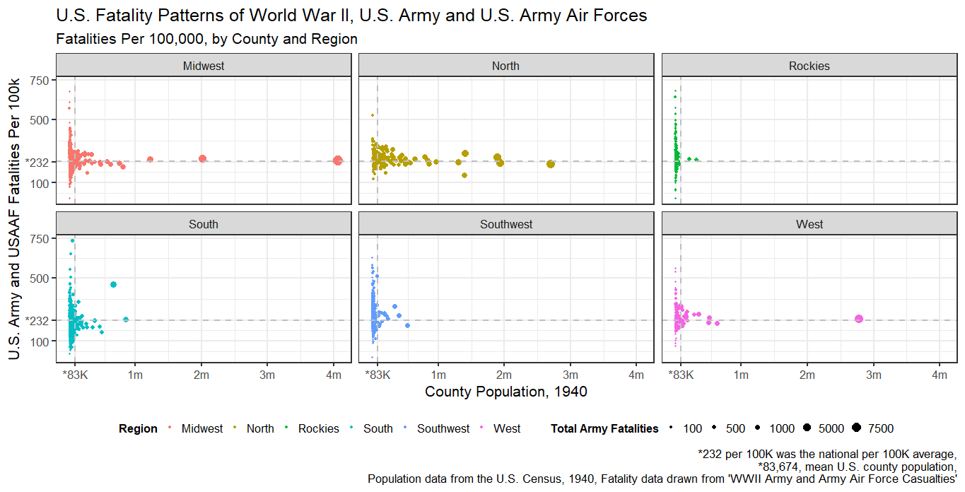
These regional trends began to change first with Korea and then with Vietnam, but not as dramatically as what would come later. During the Big One, of the top 50 most populated counties, 44 were within 90% (or higher) of the national per 100.² By the Korean War, it fell dramatically to 14 of the top 50 populated counties but rose again in Vietnam to 23. While the geographical spread had indeed changed by Vietnam, a number of America’s most populous counties still pulled their weight. Los Angeles (26.6), Wayne County, MI (which contains Detriot, 30.97), and Kings County, New York (52.6)³, to name a few, all nearly matched or exceeded the national average (graphic 3).

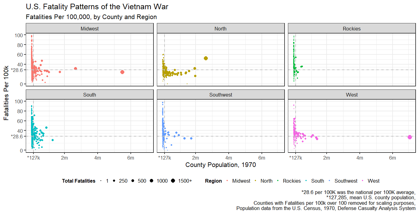
This would change dramatically with the end of conscription in 1973, coupled with socioeconomic and cultural changes associated with military service that arose thereafter. The All-Volunteer Force fundamentally transformed the face of the American military. As the Institute for Defense Analyses has noted, starting in the mid-1980s, recruitment in the Northeast dropped off the table and was largely replaced by Southern and Western states. In the wake of Vietnam, many of the North’s elite schools, including the Ivies, pushed ROTC programs off of their campuses. This slack was taken up by schools in the South and the West and contributed to the shift of identifying military service with their respective regions and political cultures.

The result was the accelerated decline of relative military fatalities from America’s most populated places, especially in the North. Only three of the 25 most populated counties during WWII failed to hit 90% of the national per capita average (Bronx County, St. Louis, and Harris County, Texas, 144, 200, and 200, respectively). If we fast forward to the Global War on Terror, only two of the 25 counties exceeded the national per capita average of 2.10 per 100k (using the 2020 census). See graphic 4.

Those two are Erie County, New York, which lost 27 of its residents (2.27 per 100k), and Baltimore City, which lost 25 (4.25 per 100k). Both are “Rusbelt” cities (the former contains Buffalo) that have bled off residents and their respective industrial bases. The economic landscapes of these counties, like rural areas, incentivized military service.

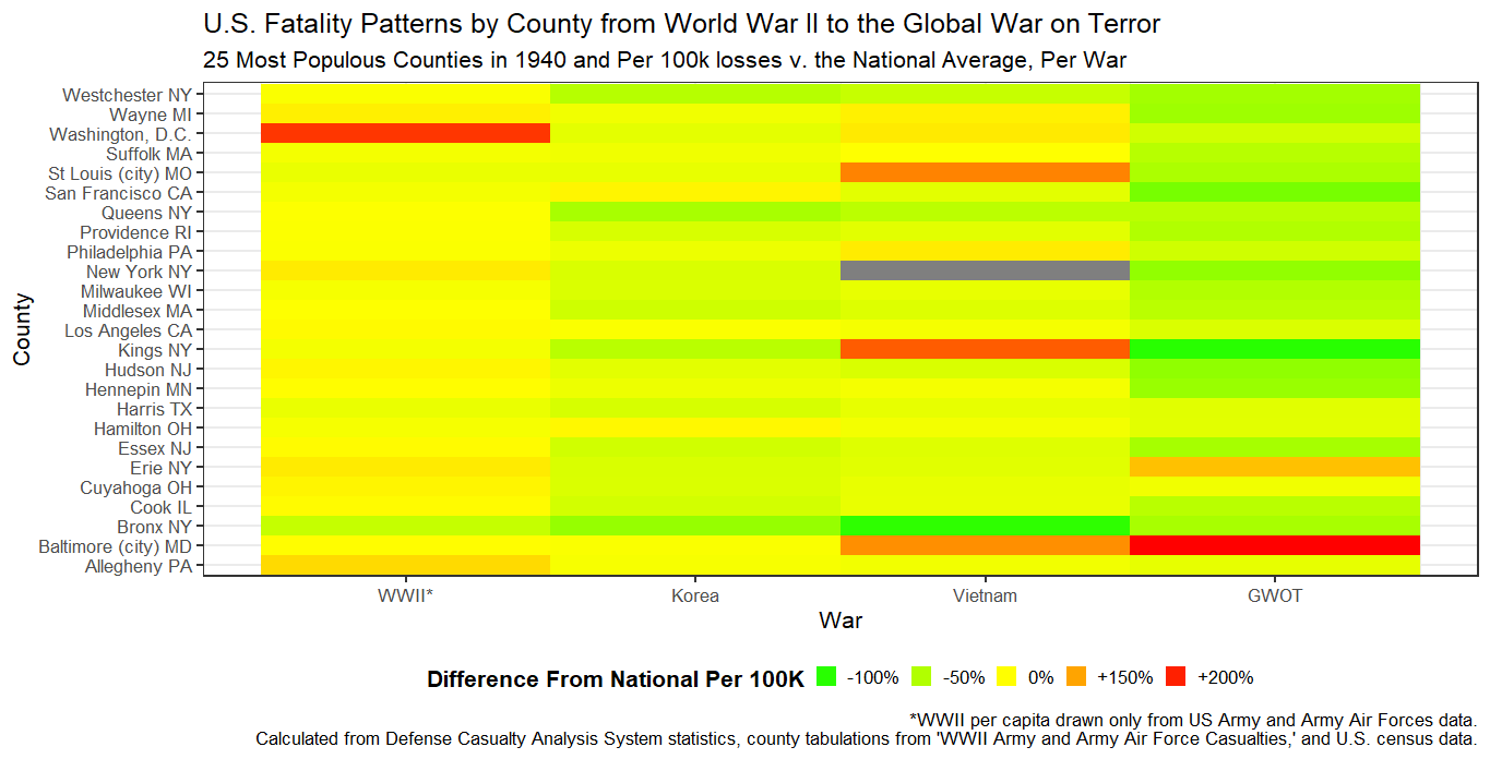
The trend is reinforced by looking at modern population data. Of the 50 most populated counties in the United States (as defined by 2020 data), only seven met or exceeded the national per capita of military fatalities endured in the Global War on Terror. Two of them, San Diego, CA, and Bexar, TX, are military towns, examples of America’s now strained multigenerational military caste.

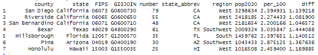
These transformations have pushed the burden of military fatalities down to less populated counties in the suburbs and exurbs (graphic 5). It should be noted, though, that most large counties still have lost a number of their resident in absolute terms. Los Angeles sacrificed 158, Cook County, 61. Yet these fatalities have been absorbed by massive populations and obscured by the growing socio-economic divide associated with military service. And, in an extreme example, Kings County, New York, population 2.7 million, lost no one in the Global War on Terror.

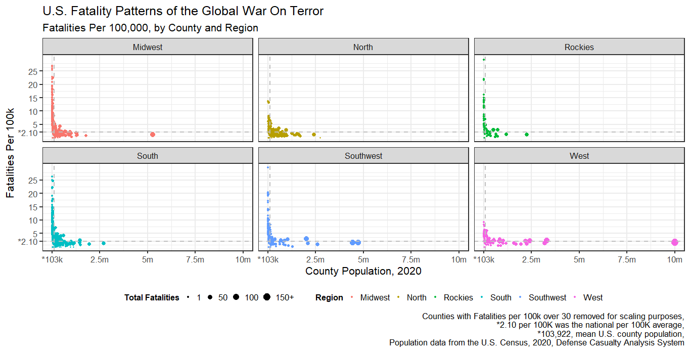
And now for the not-at-all controversial topic of race.

Remember earlier when I noted that the South lost significantly fewer of its residents relative to its population during WWII? Well, there is a reason for that: racism. A combination of exclusionary practices with the draft coupled with a general antipathy towards black combat troops meant a low number of black American wartime fatalities. Despite a number of notable black combat units in armor, infantry, and aviation, a relatively low number of black Americans died in WWII, an estimated 708.

I say estimated because, interestingly enough, the Army fatality records do not record the race (or sex, for that matter) of the deceased. Therefore, tracking racial statistics (an already fraught practice) is especially tough, and it is made tougher still given the black-and-white manner in which racial statistics were gathered in the U.S. in the 1940s (pardon the tasteless pun). Adding to the confusion was the ambiguity of Latinos in the American racial hierarchy of 1940. Latinos were, however, classified as white and served in integrated units.

Yet, if we plot per capita losses against the white population percentage, the South had a lower per capita loss rate as a region because half of its population was (largely) barred from combat (graphic 6). There were outliers, of course, particularly for a few counties in Virginia, but the general pattern holds.

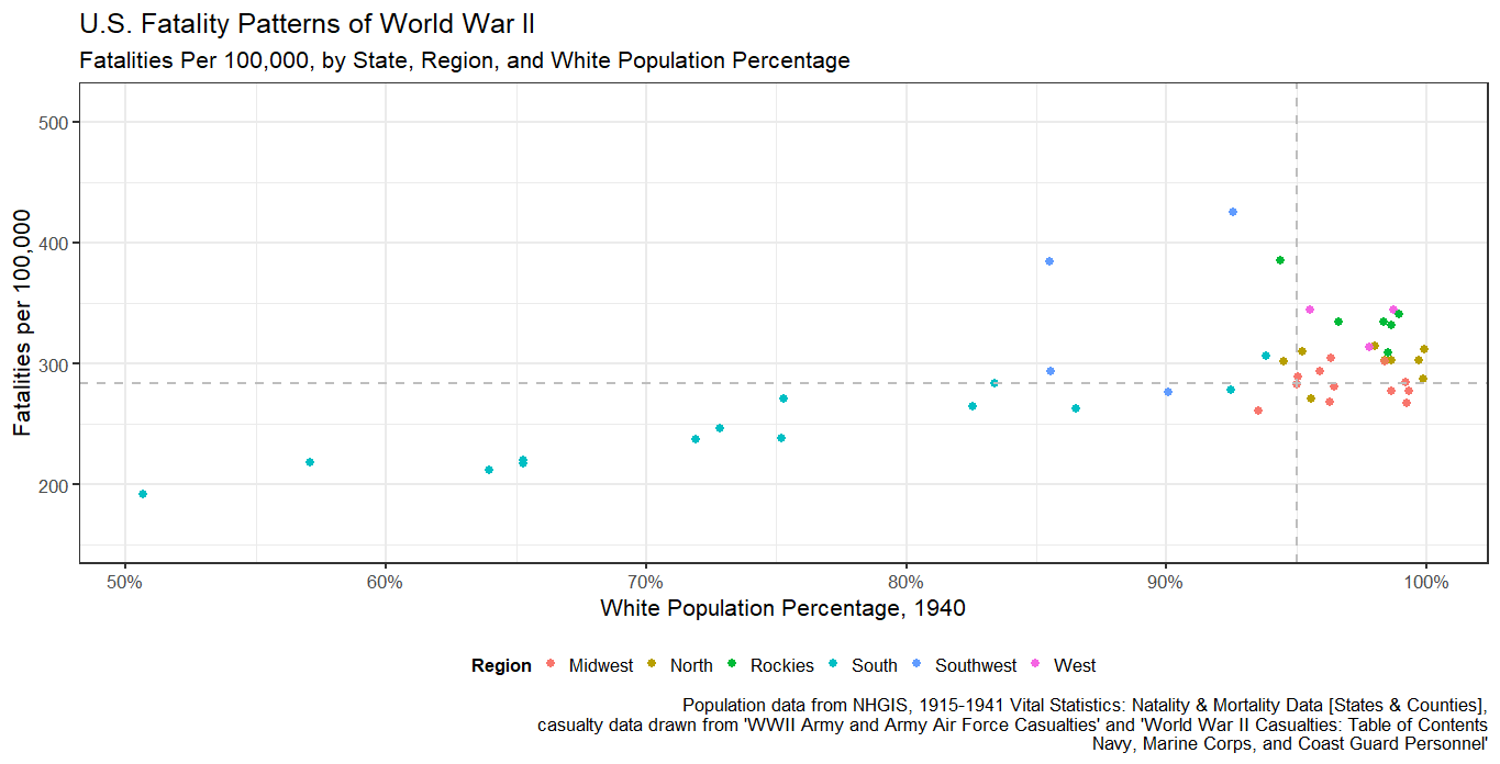
The racial patterns of American combat changed after WWII with the continuation of the draft coupled with the integration of the military. While comparisons across time are difficult due to the changing and often capricious nature of American racial statistics, looking at the DoD’s own fatality statistics, it is clear that by Vietnam, the racial breakdown of American combat largely mirrored that of the county at large (see below).

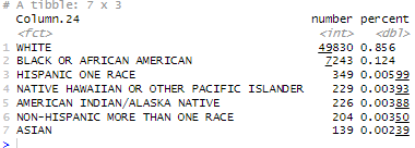
Yet, since the advent of the All-Volunteer Force, the color of combat has become increasingly white. The elimination of the draft and the adoption of volunteer enlistment coupled with a contract system have created de-facto occupational segregation within the U.S. military, a fact that the Army has itself lamented (if for its own political reasons).

This systematic difference in career paths has led to racial disparities in fatalities endured during the Global War on Terror. As the Department of Defense has acknowledged in its own reporting and its own statistics, around 70% of the country’s GWOT fatalities are white, which is higher than the U.S. military and the nation at large.

There are exceptions, of course. While the DCAS data does not list racial statistics for individual soldiers, the records themselves are enlightening. Looking at the names of the fallen in heavily Latino counties, like Los Angeles, reveals a preponderance of Hispanic surnames, and Baltimore, a predominately black city, lost 32 of its residents, a per capita of 4.2, double the national average.

Yet these are the exceptions that prove the rule: America’s combat fatalities, for the first time since WWII, have become disproportionately white even as the military and, indeed, the country at large are becoming less so. They’ve also become disproportionately rural and underrepresented among America’s upper class. Long gone are the days of UCLA or Harvard sending its students and faculty to fight America’s wars.

The elimination of the draft, moral considerations aside, constructed a military caste within the United States, one served by a volunteer system. After 20 years of lost wars and amplifying domestic issues, that system is heavily under strain. As I argued in my earlier piece for antiwar.com:

These disparities in wartime losses expounded upon another conflict, the culture war. Conservatives, who are overrepresented among veterans, have come to view the foreign policy class and similar coastal elites (to include large swaths of the GOP) with abject disdain. While it is true that the US has been awash in militaristic pageantry since 2001, the right sees the national mood as inherently hostile if not downright contemptuous of them and their values. In their eyes, conservative principles are routinely mocked by the same social class which has sent them or their children to die needlessly abroad. Their home states are referred to derisively as “fly over country.” They have been called “bitter clingers” and “deplorables.” Their religion and patriotism are routinely mocked, as are their cultural values on abortion and guns. Their views on constitutional government are ridiculed as both ahistorical and outdated. They are routinely labeled as racists, sexists, Nazis, homophobes, and so on. Worst of all, they are increasingly compared to those that they fought and are seen as a growing terror threat.

Bear Any Burden: Military Sacrifice and Rise of American Populism – Antiwar.com

It appears that America’s martial caste is now discouraging its sons and daughters from enlisting, draining the U.S. military’s strongest enlistment pool. Now, the smart set, on both the right and left, is floating the idea of bringing back the draft, often invoking World War II nostalgia, framing conscription as a form of “democracy.”

It should go without saying that the United States is not the same place that it was in 1940. Reinstating the draft would create more problems than it would solve. There is, of course, another less draconian solution to the question of who shall bear the burden of America’s future, one rarely floated by the smart set: lighten the load.

Lower the demand by bringing our troops home, make America’s “allies” pay for their own defense, and return to the republic we’re supposed to be. It’s a novel and perhaps impossible idea, but one worth clinging to lest we resign ourselves to future generations buckling under this imperious burden.

1. Steven Manson, Jonathan Schroeder, David Van Riper, Katherine Knowles, Tracy Kugler, Finn Roberts, and Steven Ruggles. IPUMS National Historical Geographic Information System: Version 18.0 [1915-1941 Vital Statistics: Natality & Mortality Data [States & Counties]]. Minneapolis, MN: IPUMS. 2023. http://doi.org/10.18128/D050.V18.0 ↩︎
2. I used this cut-off for World War II in order to account for the likelihood that naval losses would have put a given country over the threshold of meeting the national average. ↩︎
3. That number is likely inflated by an error in the DCAS dataset, one that did not record deaths for New York County. I suspect that residents of New York County were recorded as residing in Kings County, hence the elevated number. ↩︎
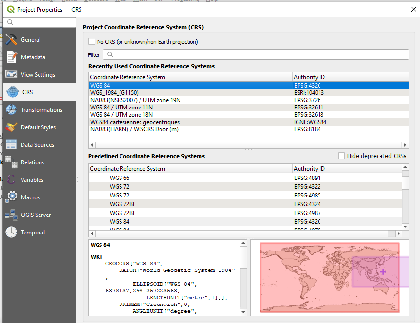
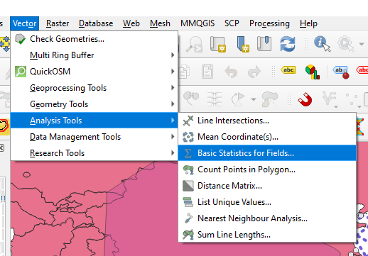
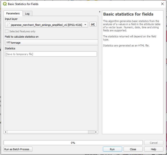
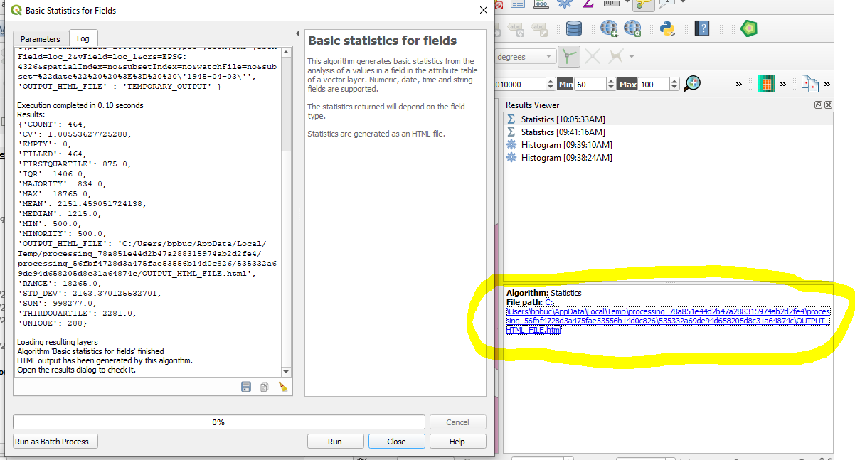
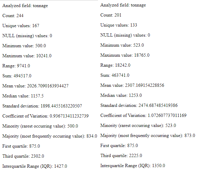
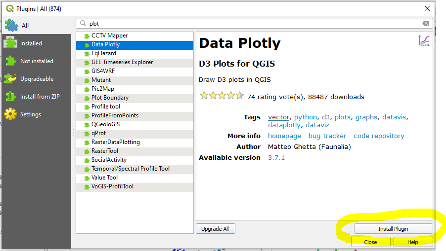
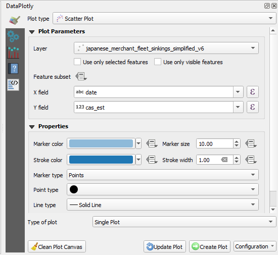
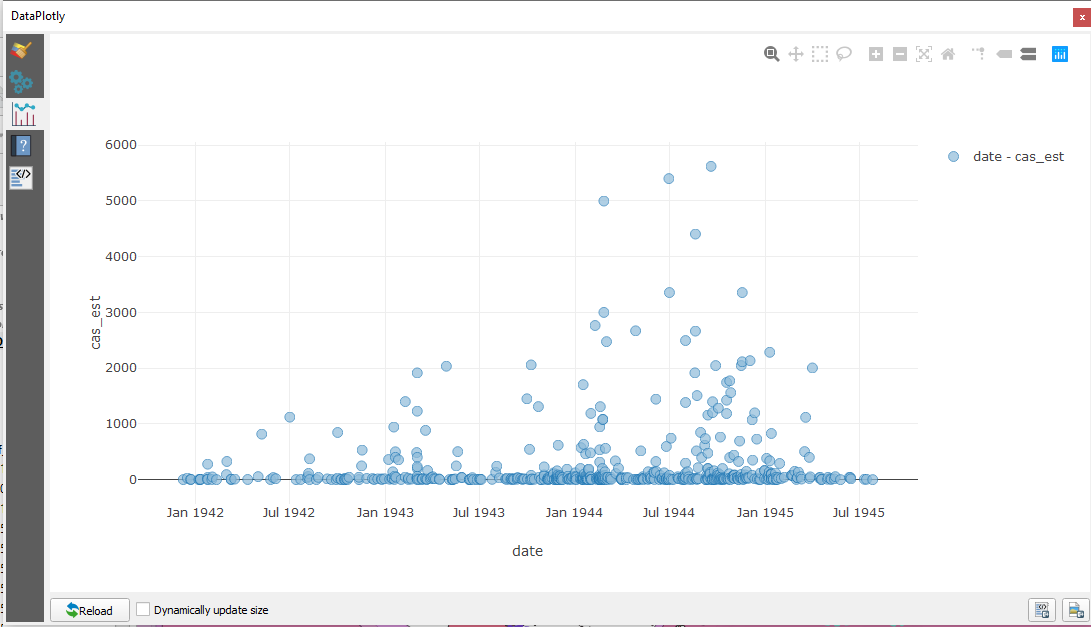
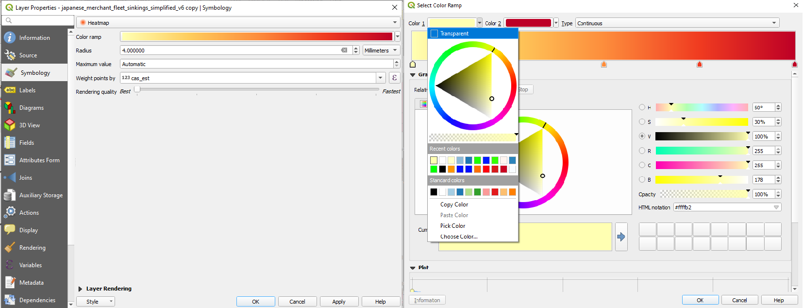
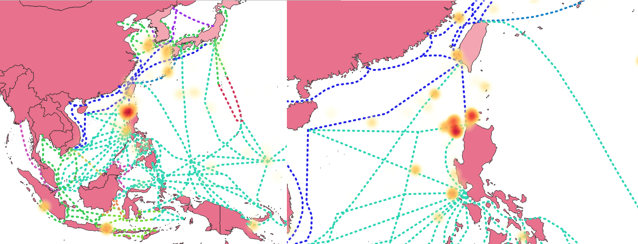
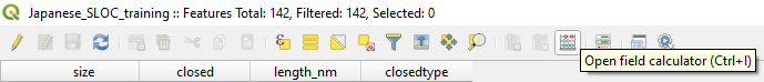
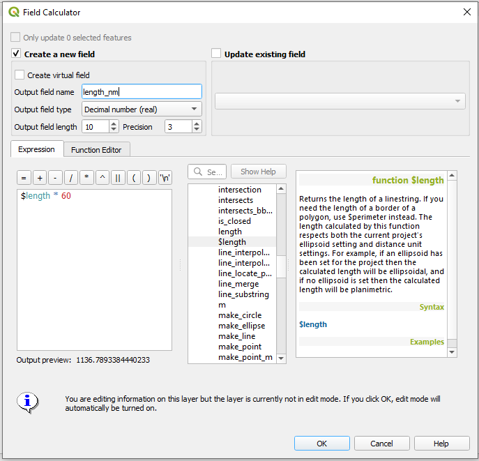
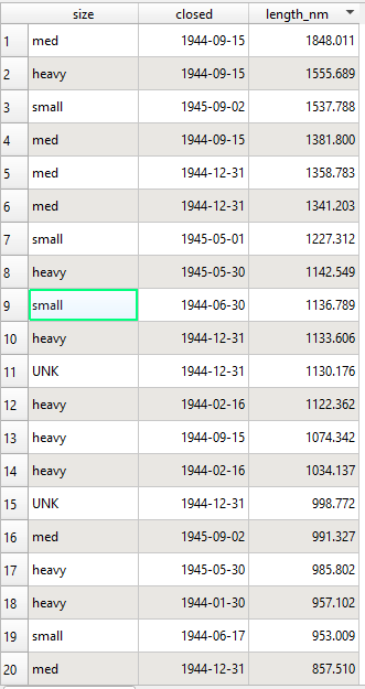
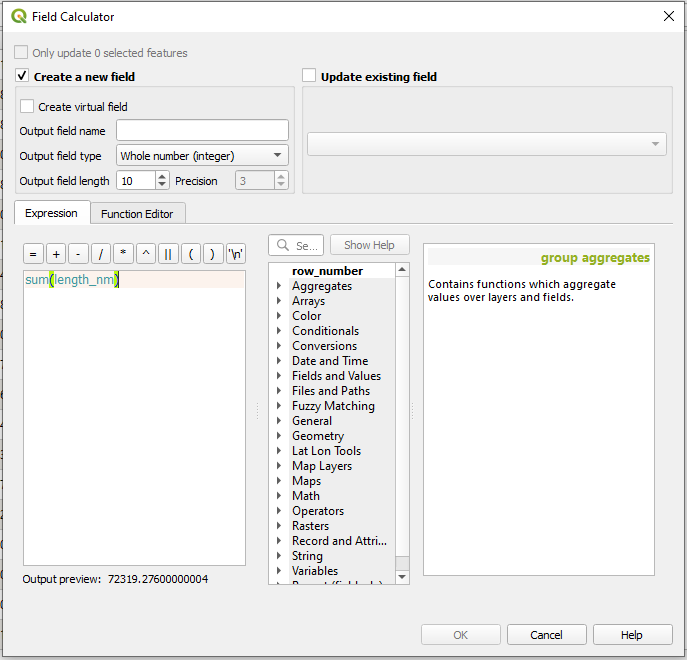
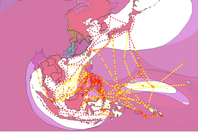
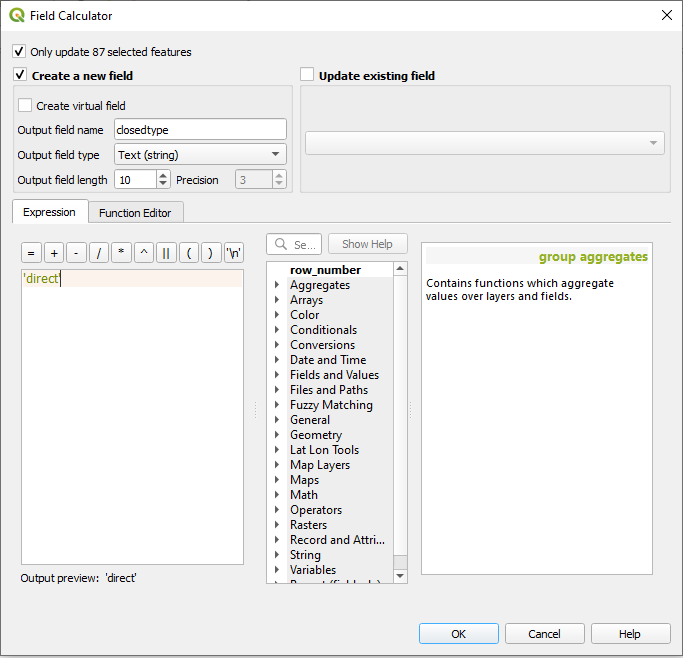
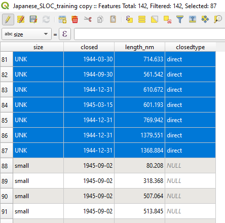
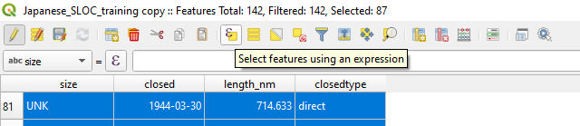
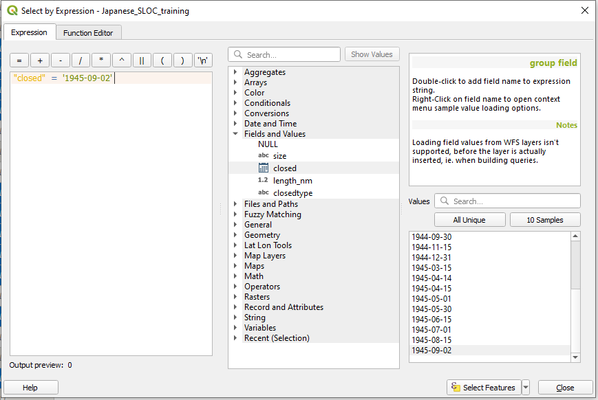
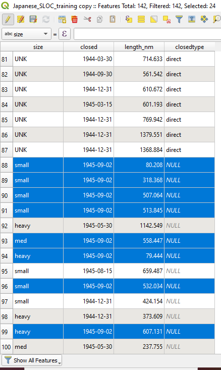
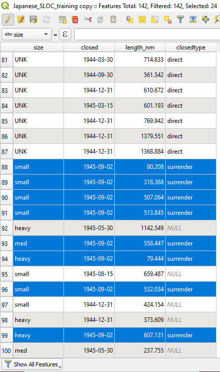
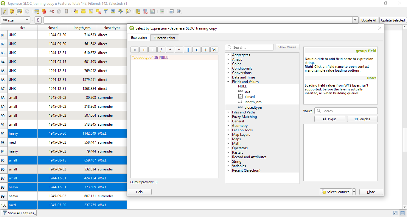
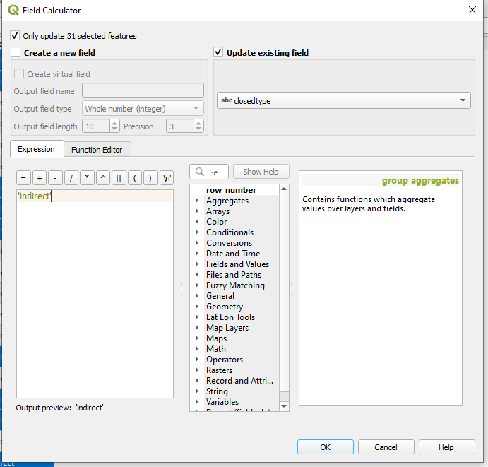
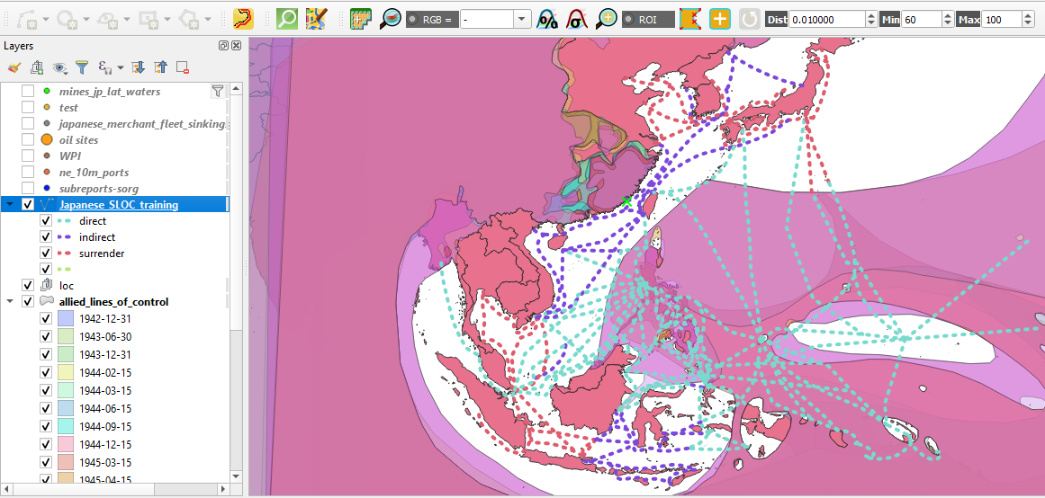
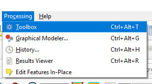
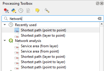
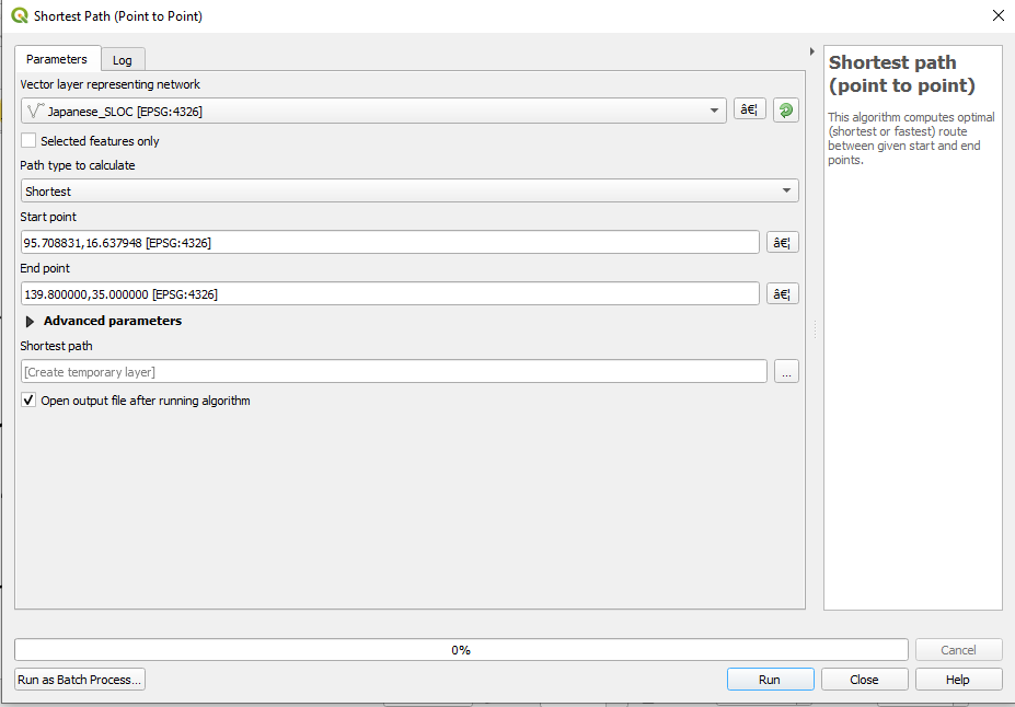
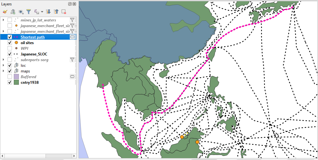
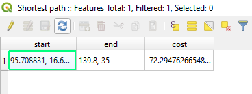
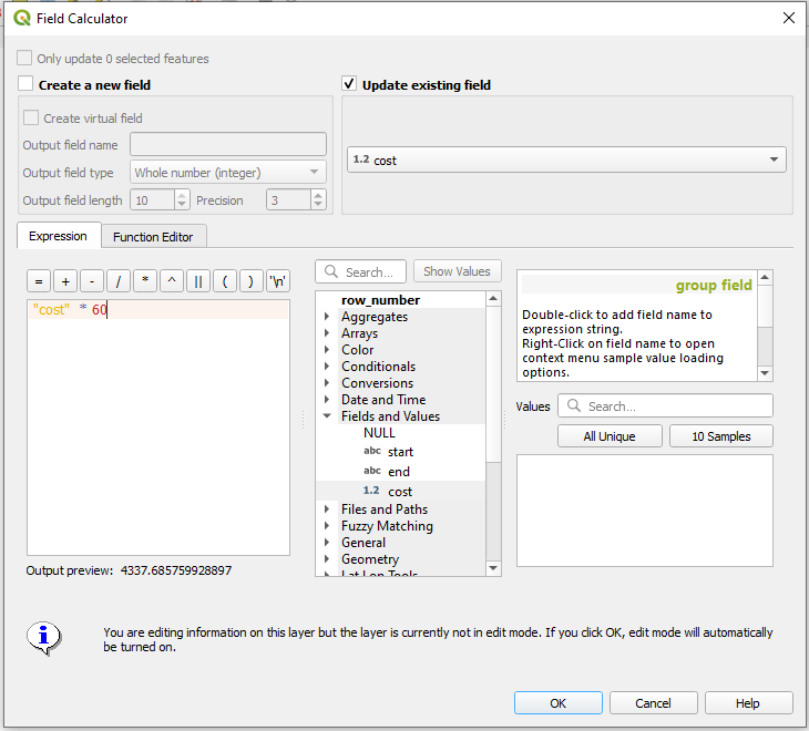
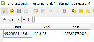
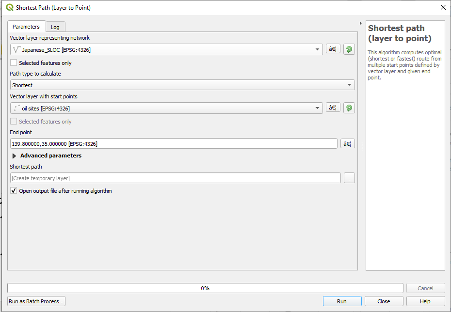
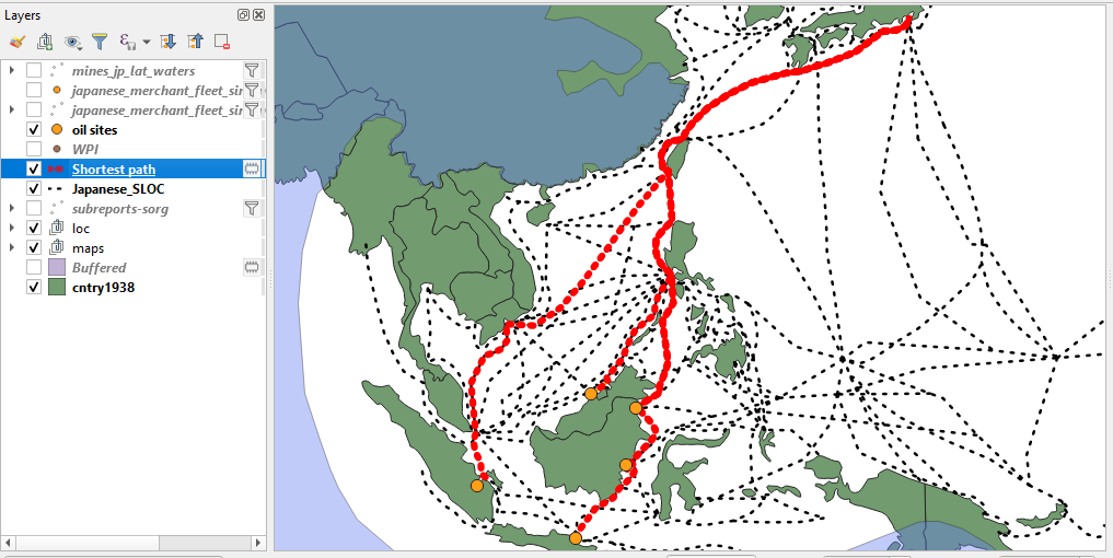
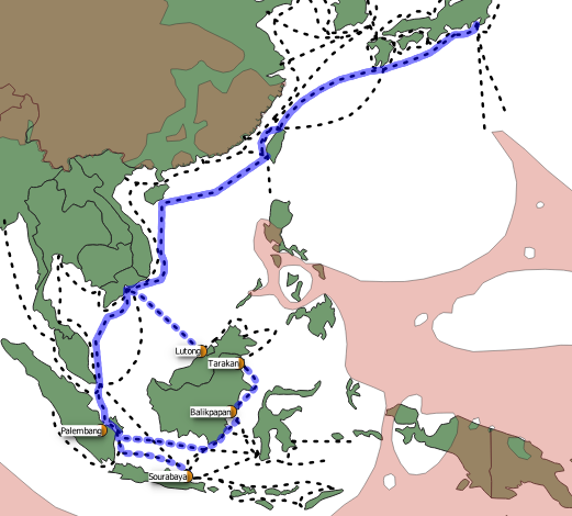
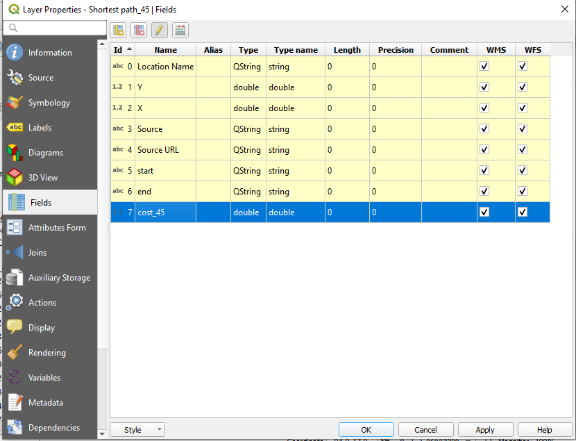
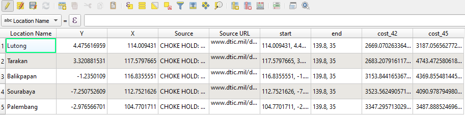
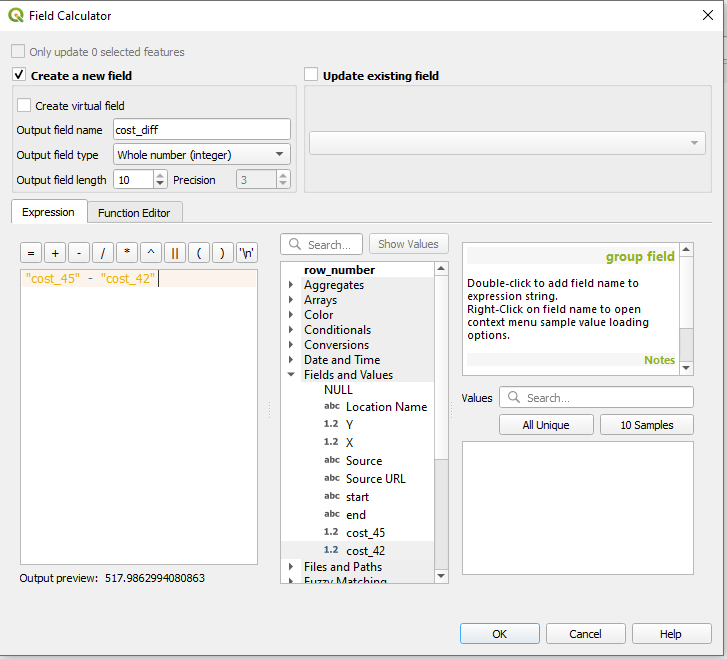
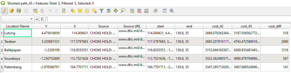
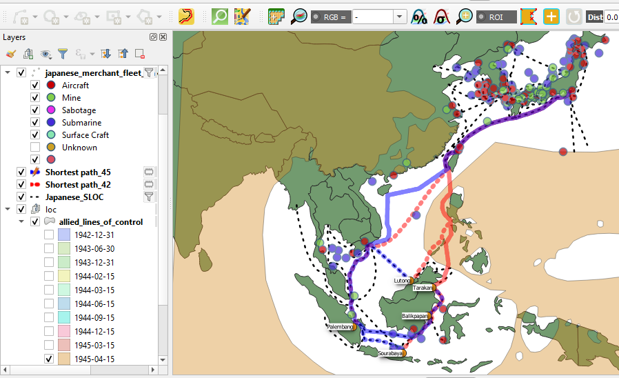
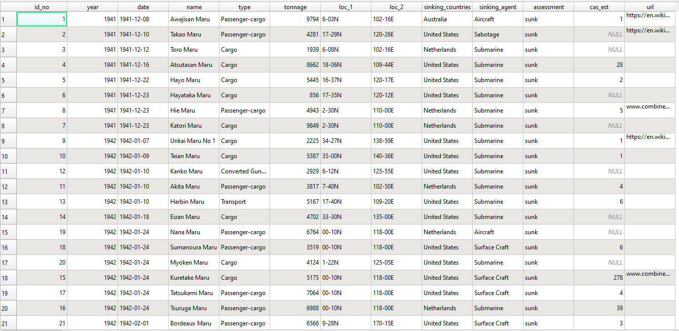
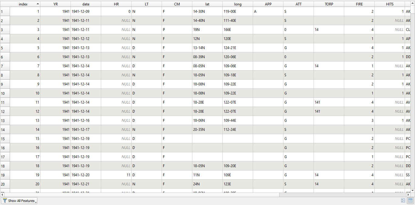
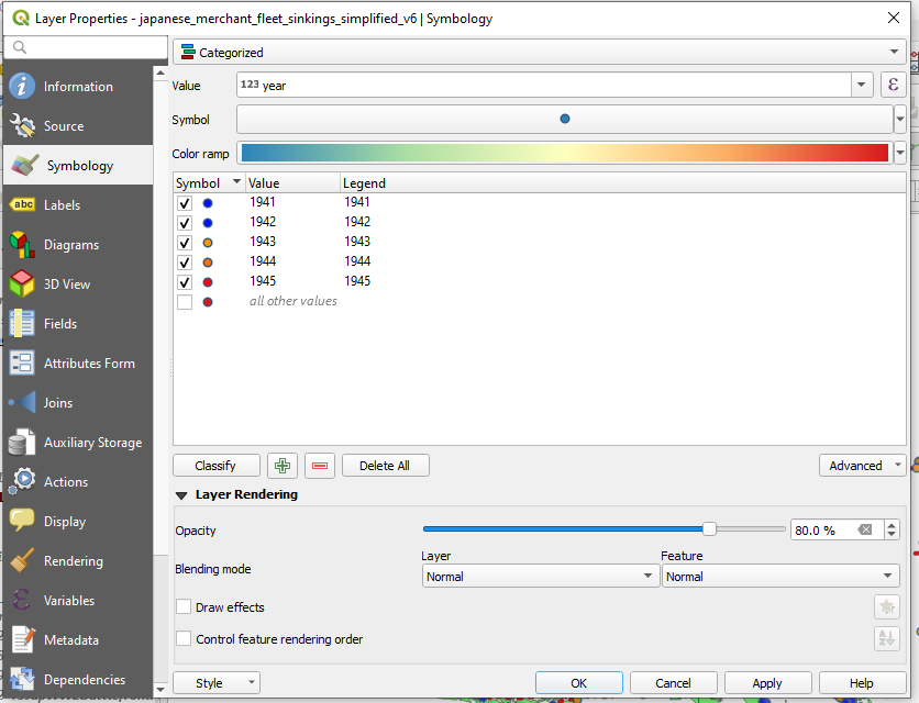
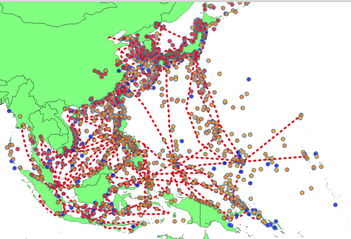
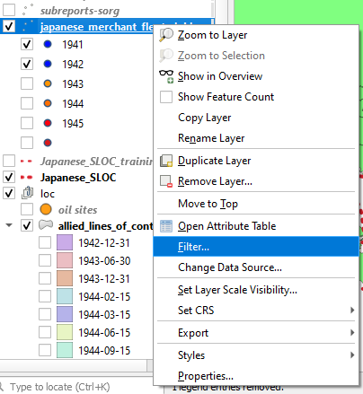
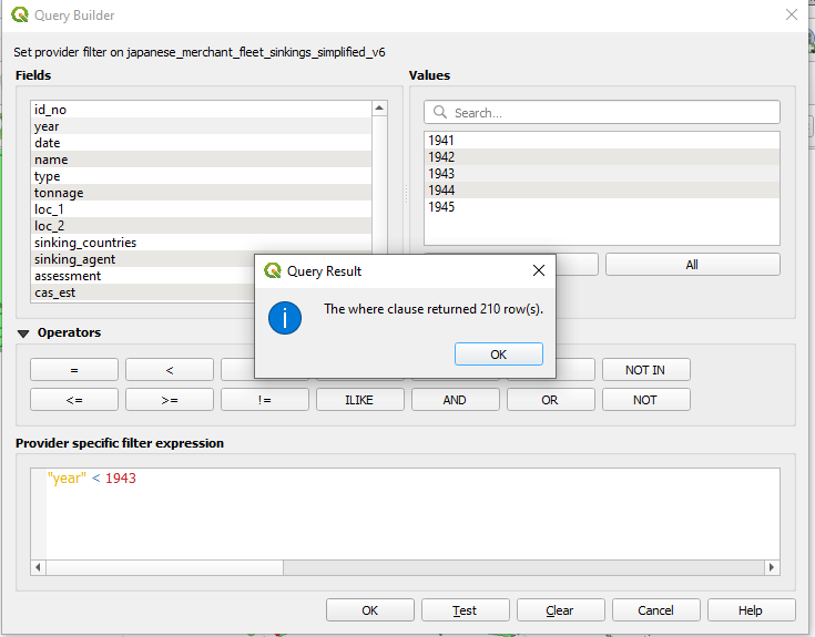
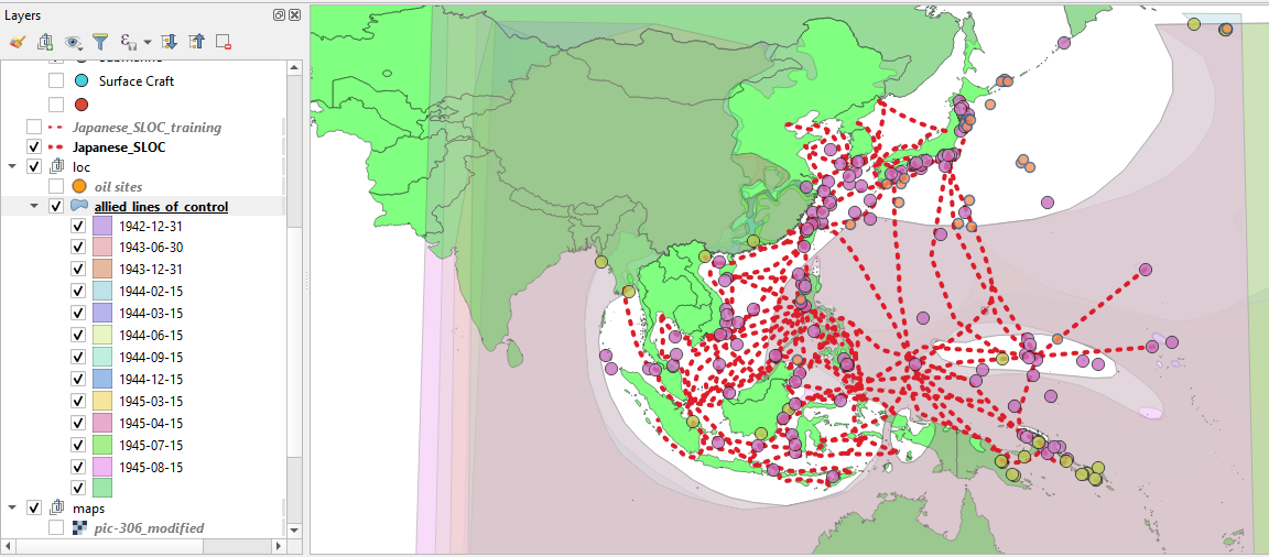
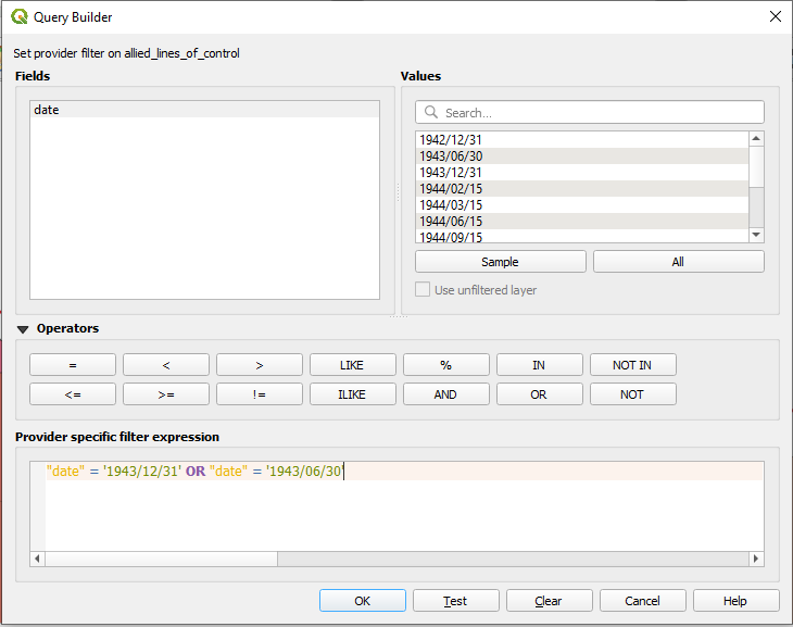
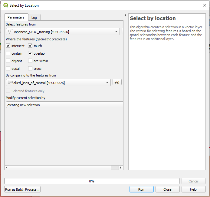
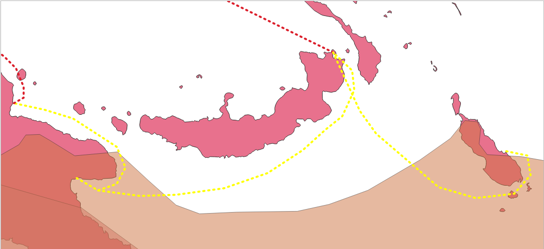
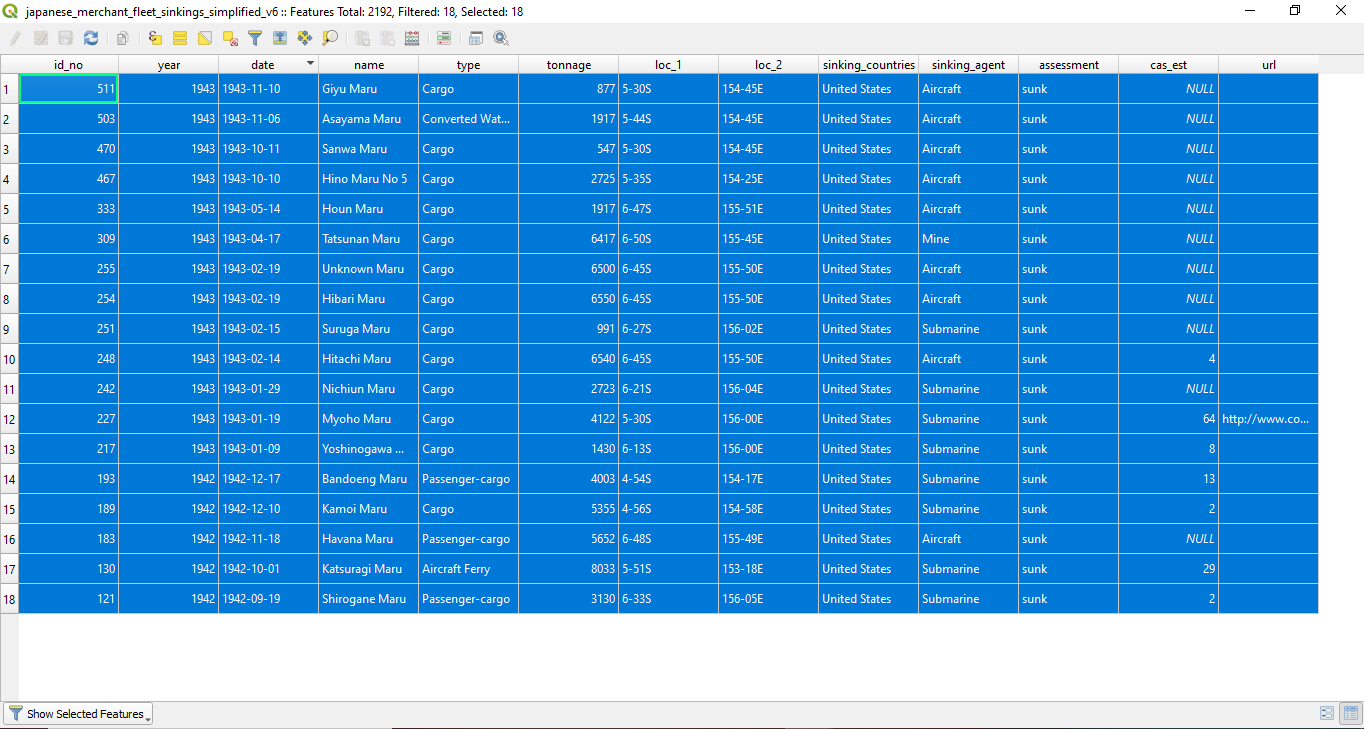
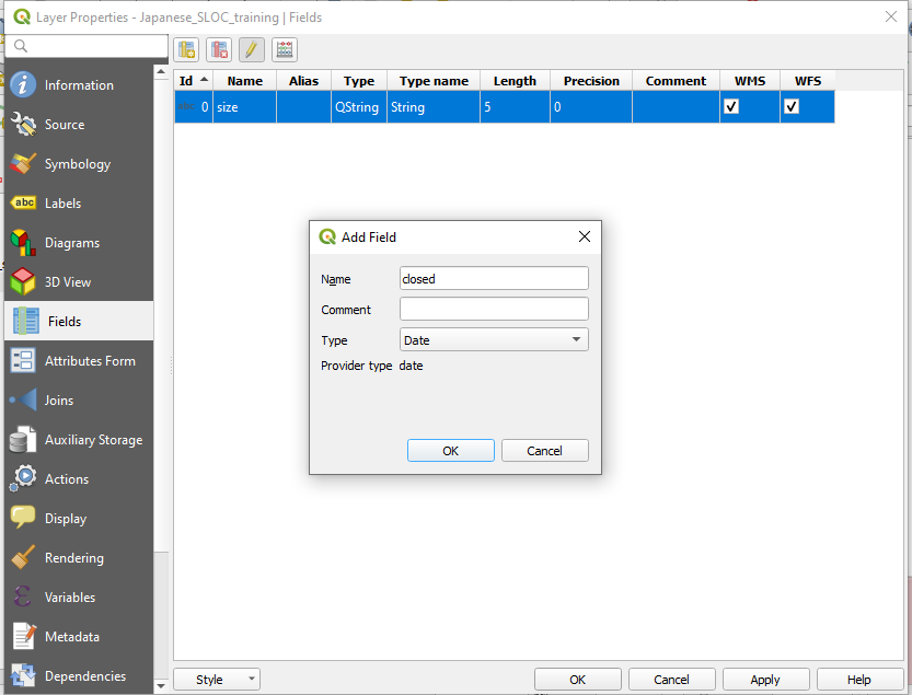
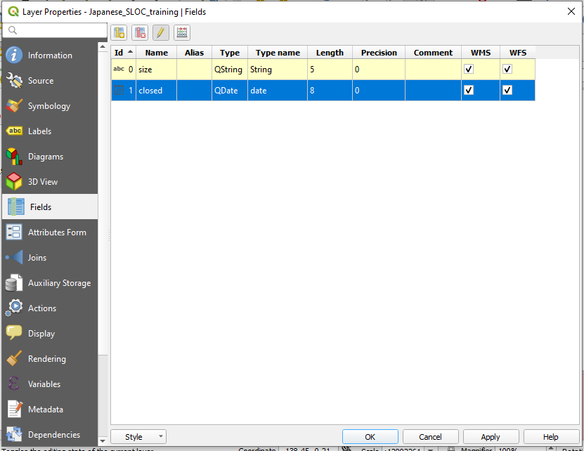
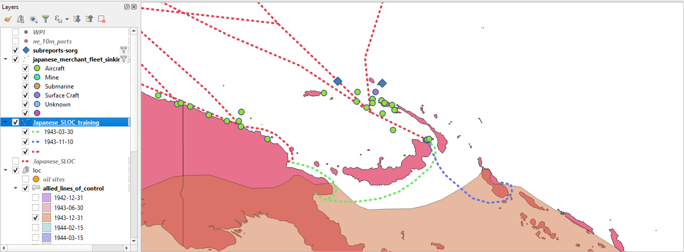
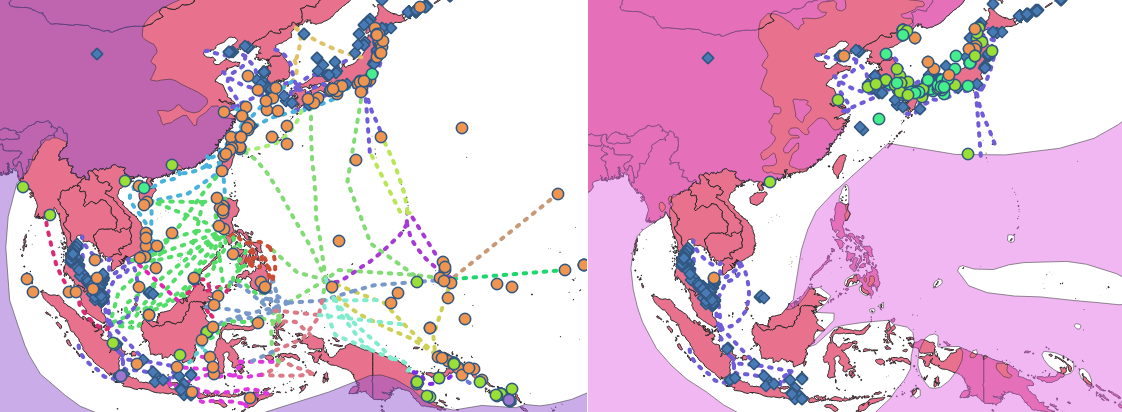
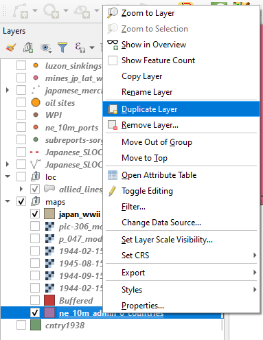
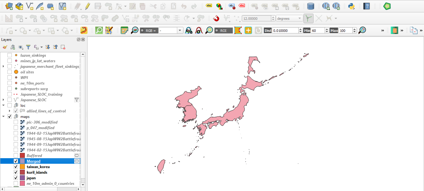
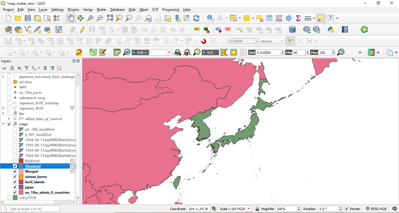
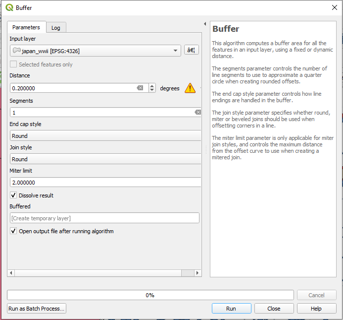
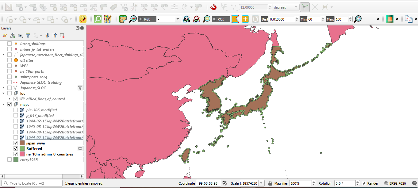
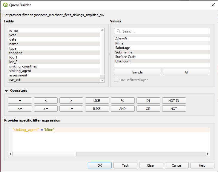
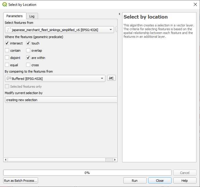
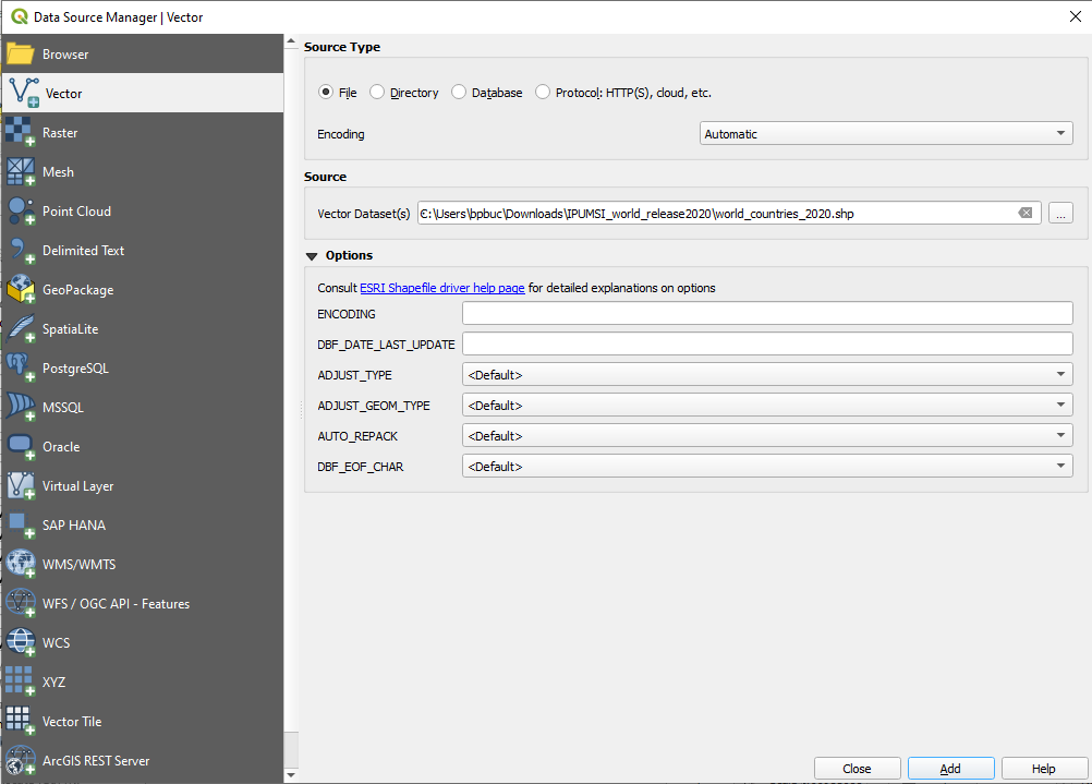
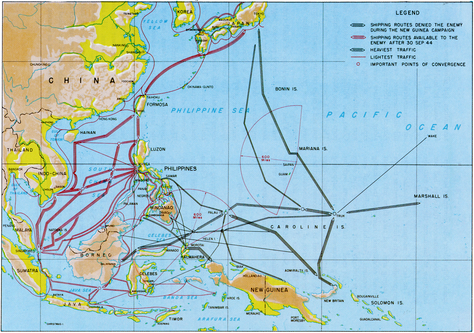
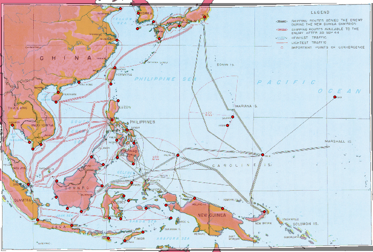
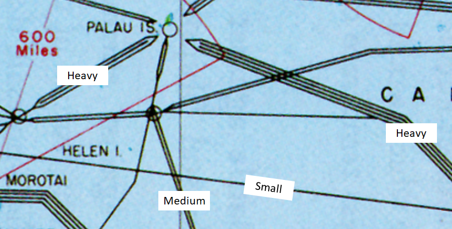
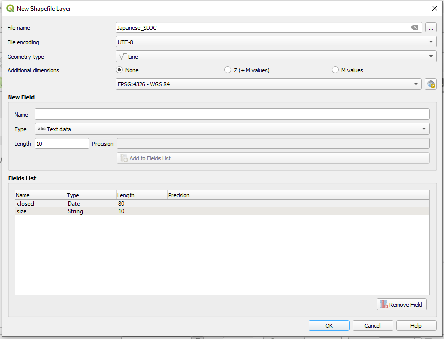
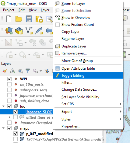
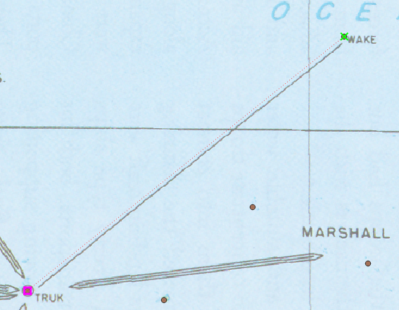
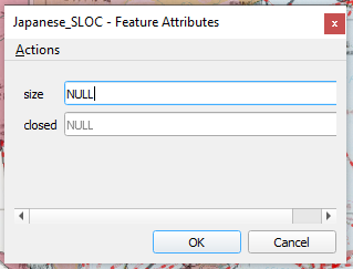
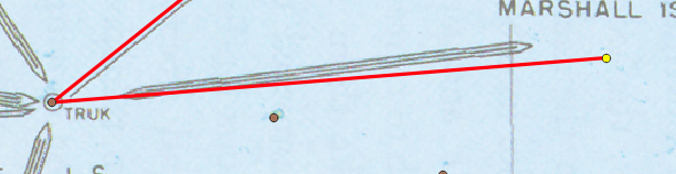
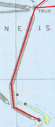
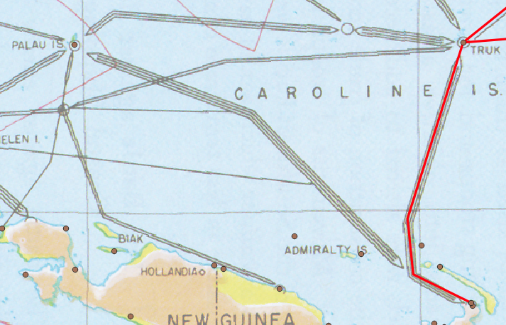
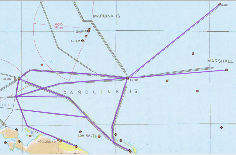
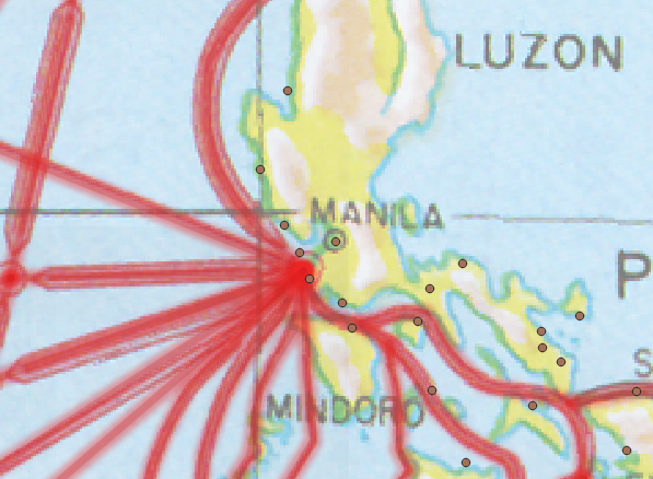
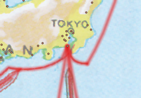
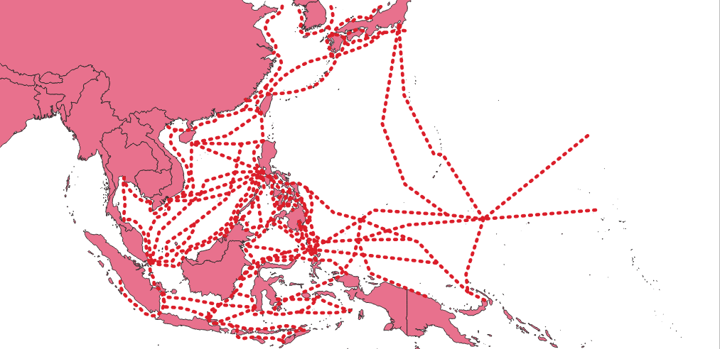
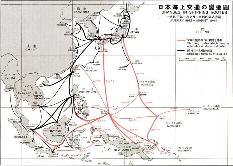
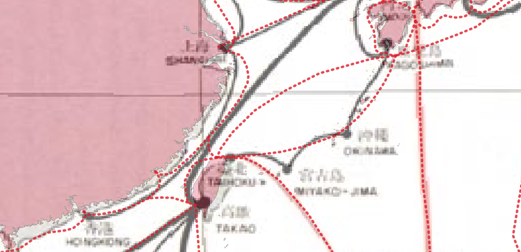
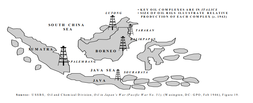
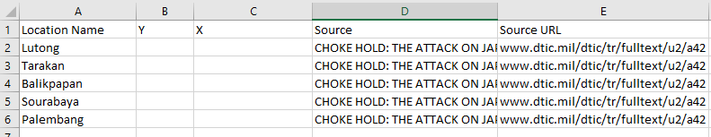
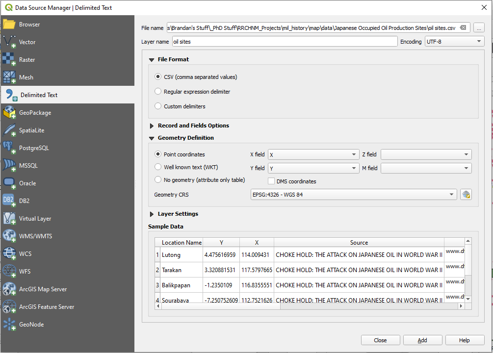
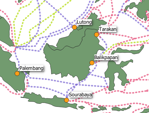
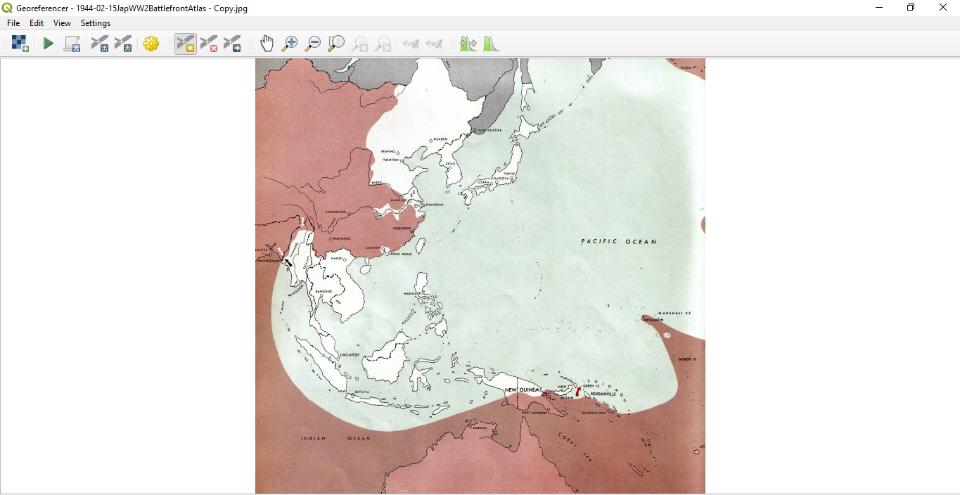
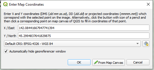
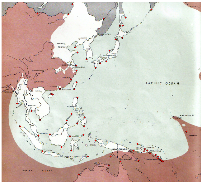
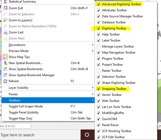
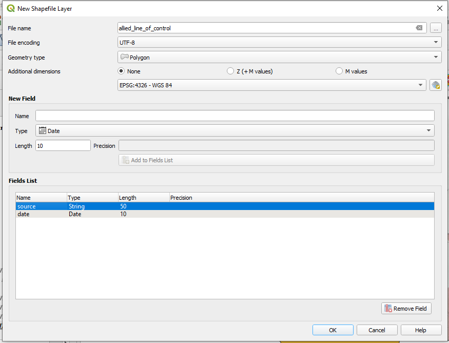
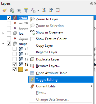
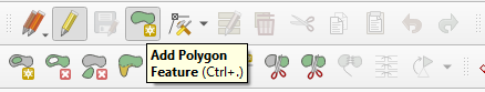
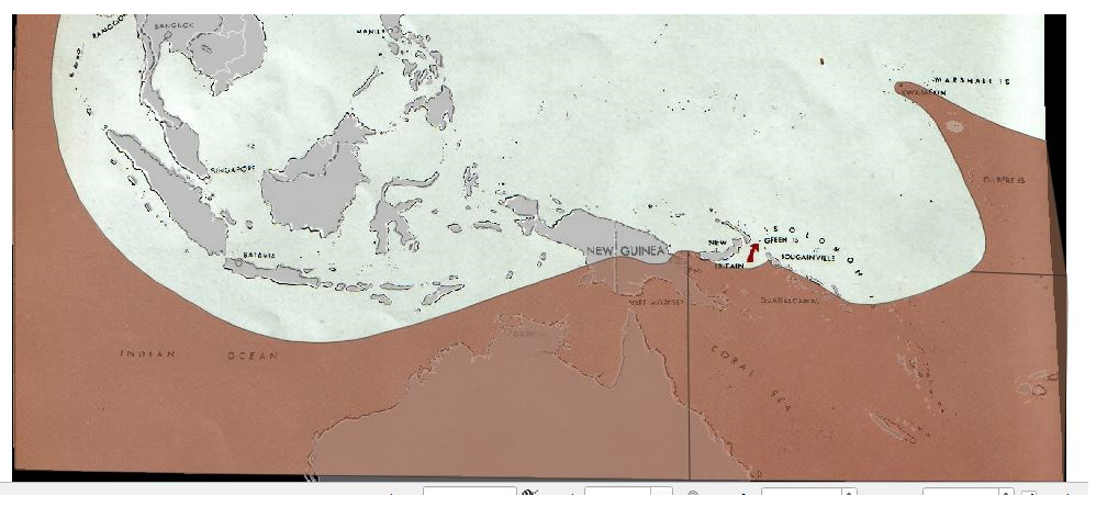
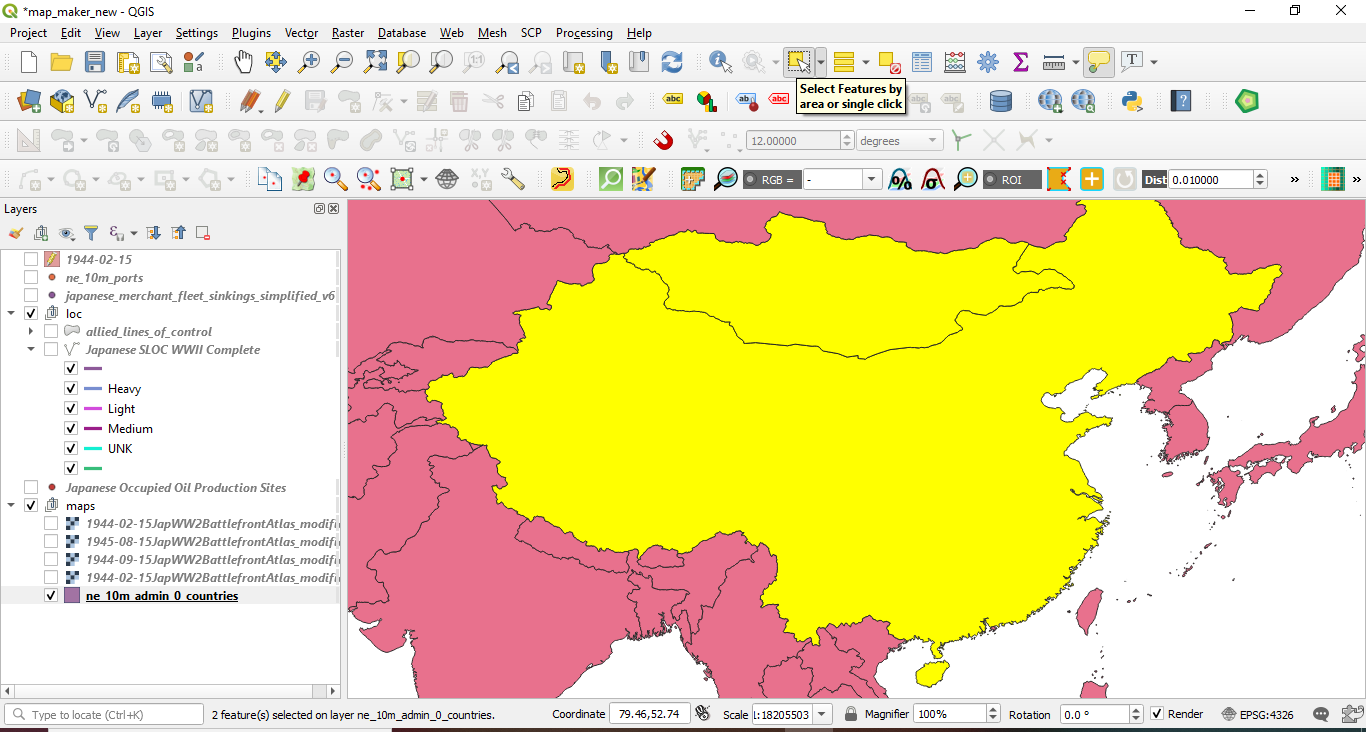
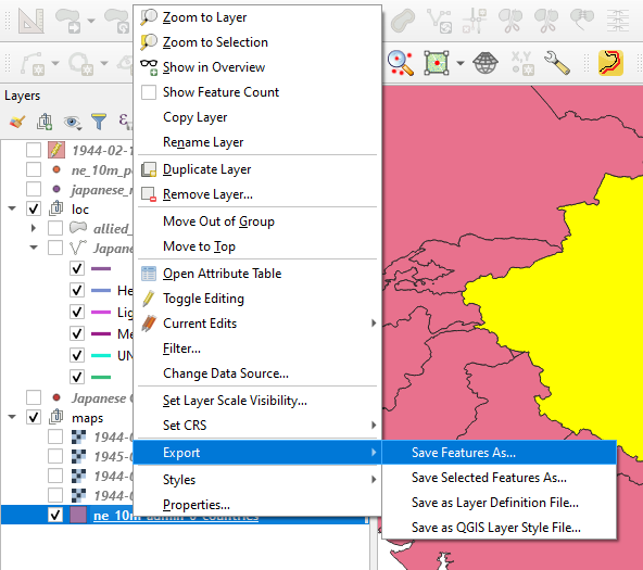
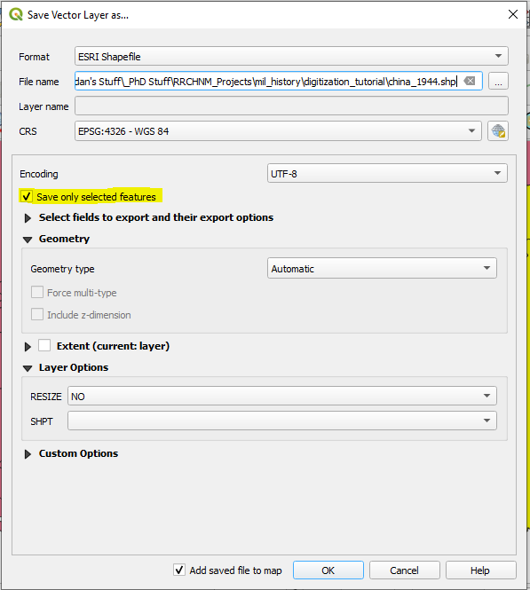
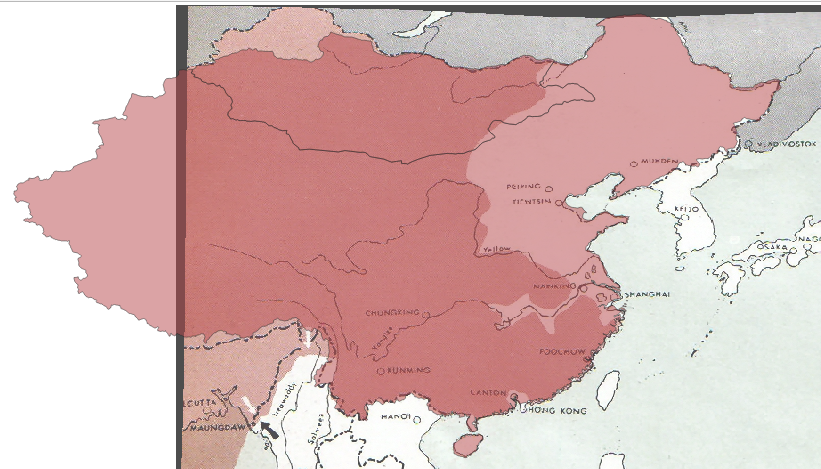
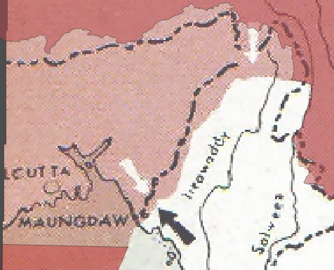
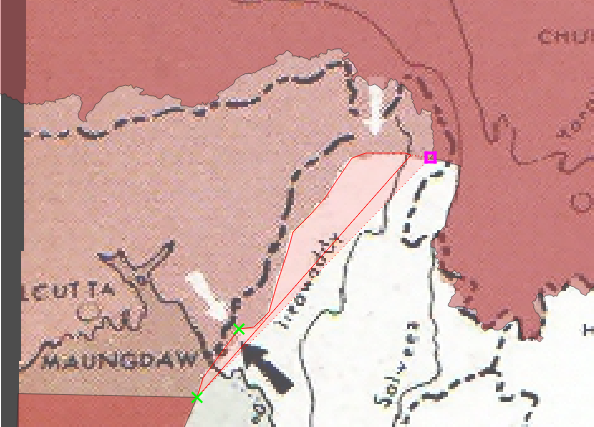
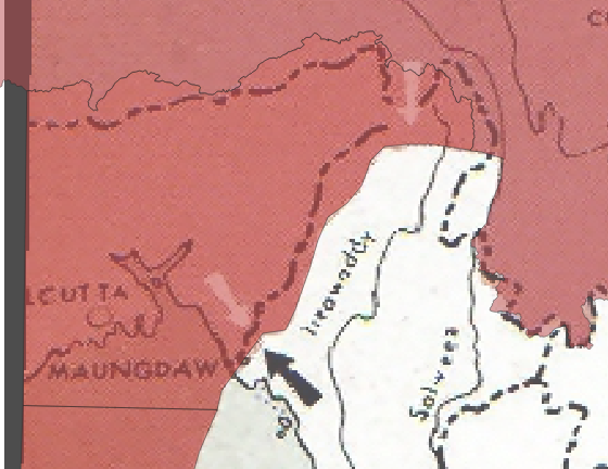
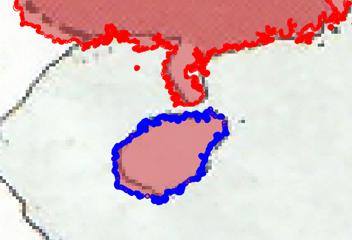
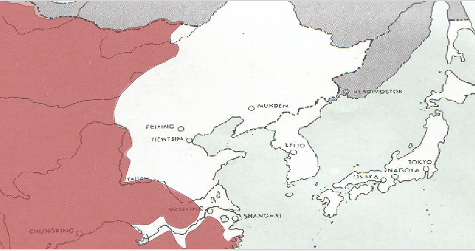
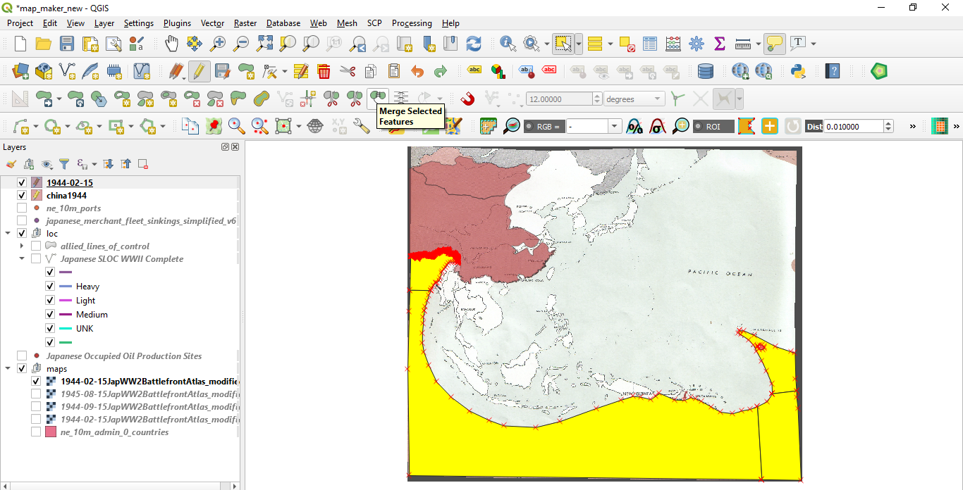
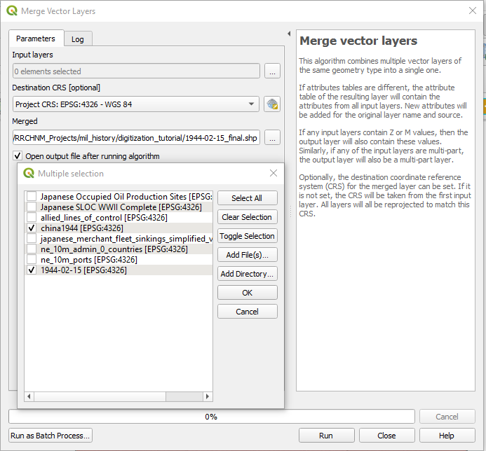
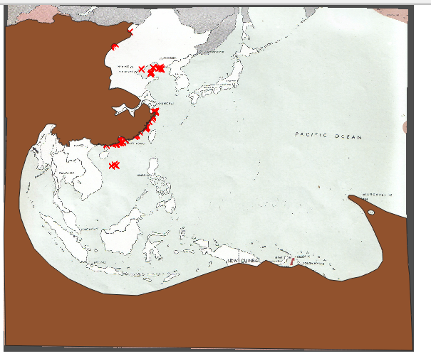
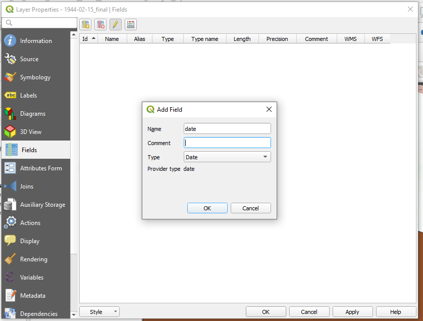
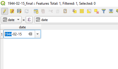
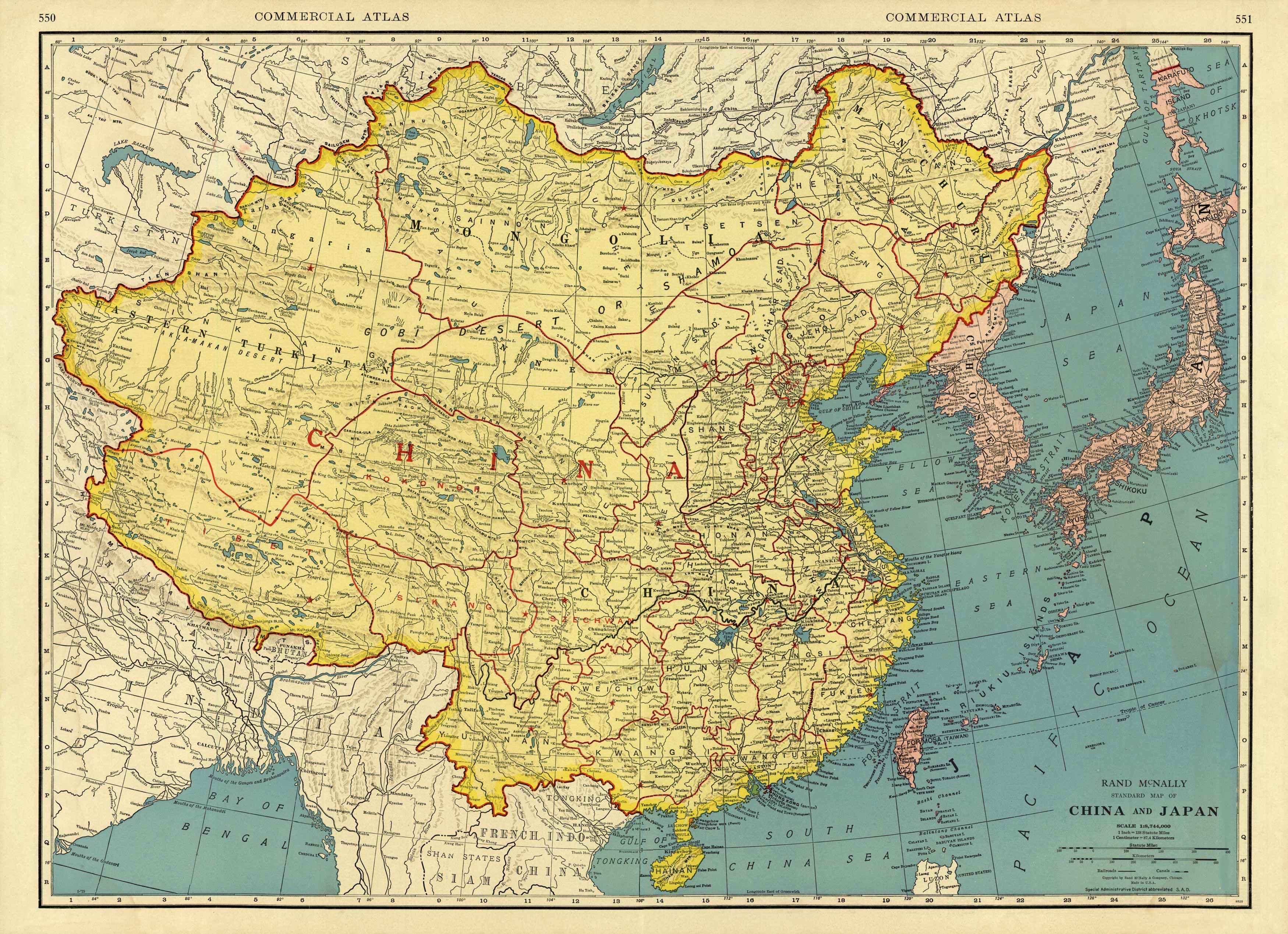