The following is the first among a series of blog posts designed to capture the lessons learned during the creation of “Unrestricted: The Campaign to Sink the Japanese Merchant Fleet During World War II.” The aim of this series is to pass along these techniques for students and professors of digital history in general, and digital military history in particular.
The first blog in this series concerns map georectification and the digitization of the polygon features contained therein. While there are a number of excellent tutorials on both of these processes they often, in my humble opinion, focus on mere “buttonology.” This series intends to serve both as a means of learning the mechanics of these techniques while also illustrating how to think through complex digitization problem. It is my hope that the materials in this series will aid new digital historians in their own endeavors and spare them the headaches that I have endured during my work.
Getting Started:
This blog series will assume that the reader has set up QGIS, and possesses a basic knowledge of how the tool works. (If not, QGIS can be downloaded here. An introduction to QGIS can be found here.) For a basic rundown on GIS data types and other essentials useful for digital humanists see this excellent resource.
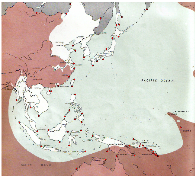
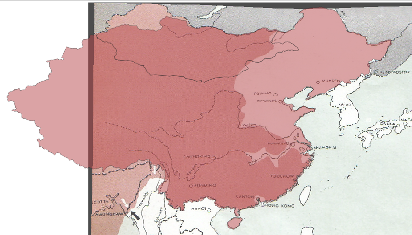
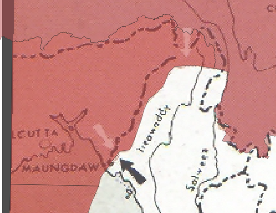
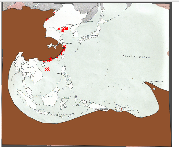
The maps which you will digitize are from The Atlas of the World Battle Fronts in Semimonthly Phases to August 15 1945 and you will be rectifying and digitizing a map from the atlas’ Pacific campaign series which depicts the state of the campaign on February 15th 1944.
You will also need a base layer with which to rectify our map. Given the scale of this project a simple shapefile of international boundaries, either from the present or the period. Either will suffice although the current shapefile, while anachronistic, contains more accurate geometries. The landmarks which you will use you consist of shoreline features and other international boundaries defined by rivers and other natural landmarks which have remained largely unchanged and are accurate enough for our purposes.
*Note: This tutorial was generated using QGIS 3.10 in the spring of 2021. Future iterations of QGIS may contain a different interface, toolbar configuration, or other cosmetic changes. Nevertheless, the functionality of the tools and concepts of this tutorial will remain pertinent.
Step 1: Create Project
a. Create a new QGIS project.Launch QGIS.
b. Project -> New
c. Name the new project.
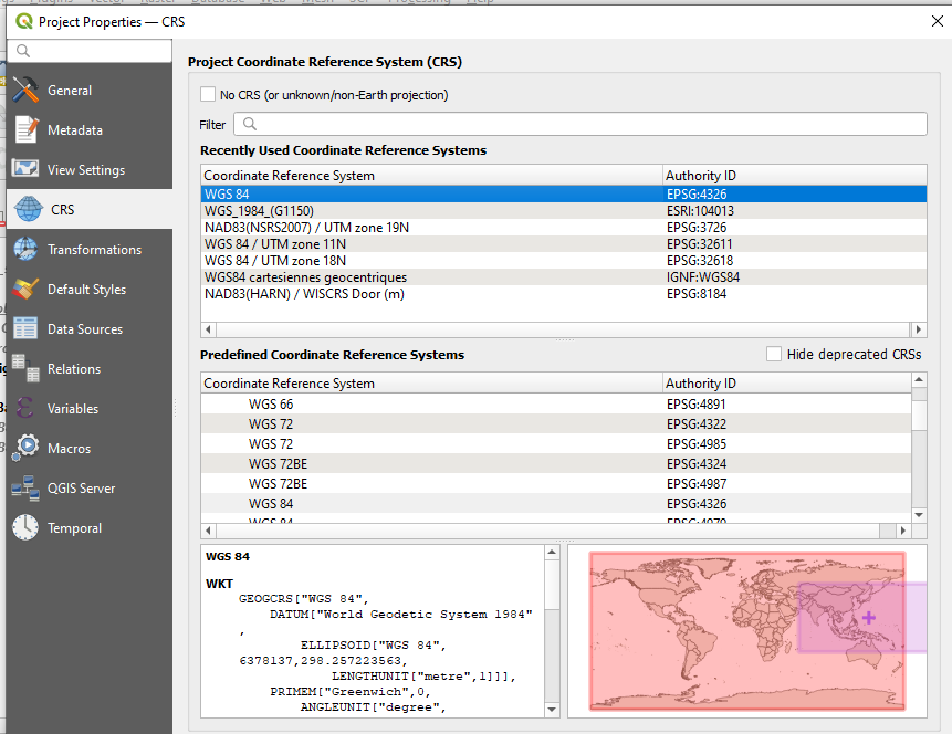
d. For this tutorial you will always use WGS 84 ESPG: 4326 as the Coordinate Reference Systems (CRS) or Spatial Reference System (SRS). To set the CRS, go to Project -> Properties, select “CRS” on the left panel. WGS 84 should be the first choice. If you don’t see it, filter for “WGS 84” and it should populate. Select it and hit ok.
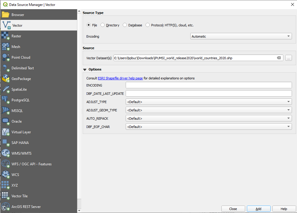
e. Add the boundary shapefile, Layer -> Add Layer -> Add Vector Layer
f. Browse to the location of the boundary shapefile, select the .shp file, select open
g. Select Add, then Close
h. Save the project
*Note on Coordinate Reference Systems. Despite the musings from some corners of the internet…the Earth is not flat. Traditional maps are a 2d representation of a 3d reality. As such, compromises must be made in order to make maps legible. Coordinate Reference Systems are a means of doing so. They define “how the two-dimensional, projected map in your GIS relates to real places on the earth.” All CRS types make compromises due to the limitations inherent to their role. WGS 84 is the mostly widely used CRS available. It is the standard for the U.S. Defense Department and is used in GPS systems worldwide. However there are examples where it can be of limited use, particularly for regions nearer of the poles of the Earth. However, given the scale of this project it will be more than adequate.

Georectify the map. The purpose of georectification is to apply geographic data to a “dumb image” thereby making it a file which can be used in a number of Geographic Information Systems (GIS) tools. This can be achieve this through a combination of QGIS’ reference tool, patience, and science! Since our goals here are to digitize historical information on a global scale our accuracy needs will only need to be good enough to accomplish said goal. You’re digitizing a war not fighting one, best not let the perfect be the enemy of the good.
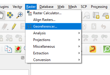
Step 2: Launch QGIS’ Georeferencer Tool, Raster -> Georeferencer
a. Open the map-to-be-rectified, File -> Open Raster, navigate to the file, select it and click open. The window should look like the one below.
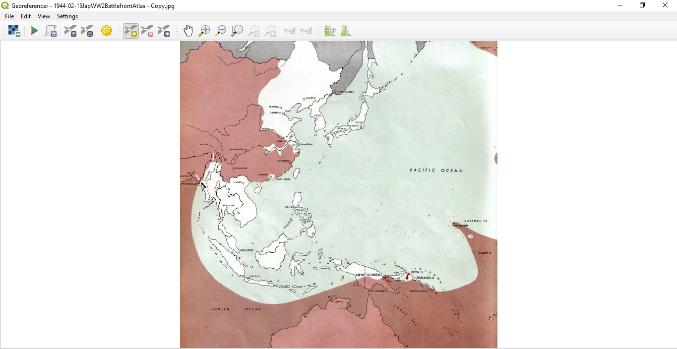
In order to complete this process you will need to manually associate points on the image to those from the base layer. Technically the process only requires four points. However, since the ultimate goal of this exercise is to digitize the crimson portion of the map which depicts the extend on the Allied advance during that period, you will need enough to ensure reasonable accuracy.
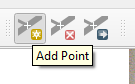
b. To start, click “Add Point”
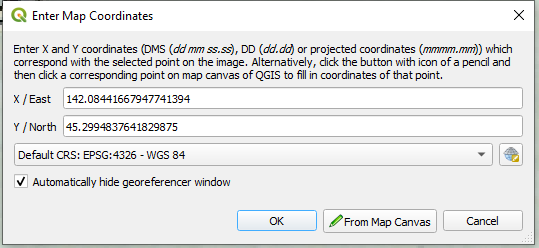
c. You will be automatically prompted to select a point on the image to rectify. Select a point on the image and you will be prompted with a window entitled “Enter Map Coordinates.” Select “Map from Canvas” at the bottom.

d. The Georeferencer will close automatically, use the cursor to select the corresponding point on the base layer. The “Enter Map Coordinates” window will reappear with the the X and Y boxes filled in.
Hit ok.
Congratulations, you’ve completed the first step on a long and tedious journey. Now would be a good time to fire up a podcast…if you haven’t already. Repeat this process until a satisfactory number of points have been created.
QGIS allows users to save the georeference points. Save them early and often. Georeferencer has been known to crash on occasion. Obsessive compulsive saving will likely save you the headache of repeating work in the event of a crash.
e. For this trial, 60 points were generated due to the map’s scale and complexity. Special attention was placed upon regions of the map which will demand greater accuracy for the purposes of digitization. Examples of such are Bougainville and Guadalcanal.
Note on points: Technically, only a minimum of four points are required, how the minimum is usually insufficient for a quality rectification. Unfortunately there is no hard and fast rule on how many it is necessary as that number is highly project dependent. Factors which can impact the the necessary number of points can be image size, detail, and scan quality. For this project a high number was necessary due to the maps relatively low resolution, the manner in which it was scanned, and its scale.
The Geospatial Historian provides some solid rules to live by.
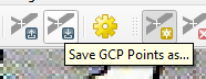
f. Now that our points are generated it is time to process the image. Click the gear icon at the top of the Georeferencer panel, it will launch a window entitled “Transformation Settings.” Choose the settings selected in the image below. Check “Save GCP points” and select the output location for output tif. Also select “Load in QGIS When Done.”
Finally…hit ok.

g. Time to check your work. You should see an image in the QGIS viewer pane and the item should appear to the left in the QGIS layers menu. Click and drag the new georectified image and drag it above the base layer (the borders shapefile). Right click on the image and select properties. Navigate to “Transparency” and crank the “Global Opacity” down to a level with which you are comfortable.
Hit ok.

f. Now that the map is semi-transparent, use pan, zoom in, and zoom out to check your work. The map’s edges will likely look warped. That is that is normal and indeed expected. However the features of the map should roughly align with our base layer. If significant distortions are noted you may have further work to do. Thankfully since you scrupulously saved your points (you did didn’t you?) you can complete further rectification by adding, deleting, or moving existing points in the Georeference tool.
You’ll likely notice that the image isn’t “perfect.” The map was not constructed to the same detail as our base layer. As such certain features, like inlets, small islands and other minor features will not align exactly. And, if you’re an astute observer you’ll likely notice that the map’s depiction of the Mongolian-Soviet/Russian border differs from our base layer as well. Despite these deficiencies the georectified layer is “good enough” to provide the data you need to digitize.

Digitizing Features on the Map.
But wait! There’s more! This would be a good time to start another podcast if needed…this may take a while.
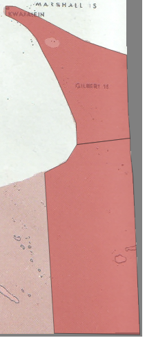
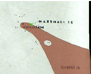
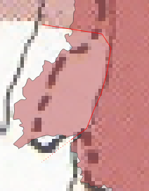
Now that the map is georectified it is time to digitize portions of interest. For the purpose of this tutorial you are interested in the crimson portion of the map which signify the extent of the Allied advance in the Pacific theatre as of 15 February 1944. This feature, which spans a large part of the Pacific poses a special digitization problem as the area depicted covers open ocean, adheres to international borders in some regions and bisects them in others. Similarly, the area you are going to digitized is often bounded by shorelines, rivers, and other obstructions.
You could simply digitize this entire area free hand. However to do so would take a prohibitively long time and likely not be as accurate as one would like.
Instead you will use a suite of QGIS’ tools to digitize certain portions by “harvesting” the existing geometries within our base layer map. You will then combine those efforts with a traditional freehand digitization.
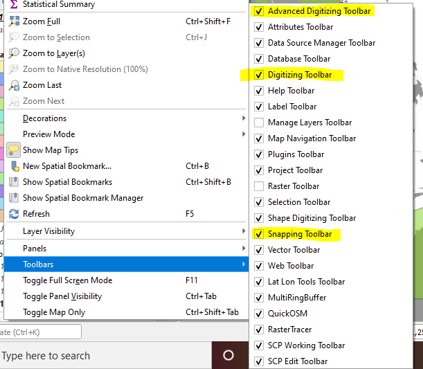
Step 1: Ensure that the “Advanced Digitizing Toolbar,” “Digitizing Toolbar,” and “Snapping Toolbar” are active.
a. Navigate to View -> Toolbars and ensure that the three tools are checked. The Toolbar menu should look similar to the image below:
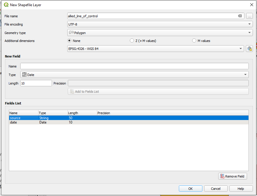
Step 2: Create a Polygon Shapefile. Navigate to Layer -> Create Layer -> New Shapefile Layer
a. Give the shapefile a name and choose a file path from the “…” button. Choose “Polygon” from the Geometry type dropdown menu and make sure “ESPG: 4326 – WGS 84” is selected. The bottom half of the window is for creating fields within the new shapefile. For this shapefile you’re going to use a simple schema, one column for the date of the map and another for the source’s name.
Hit ok.
Step 3, The “Easy Part.” I would recommend doing this in chucks and saving often. QGIS can be finicky. Losing a digitization project while on the leg can be disheartening. Also, the scale of this digitization means that you’ll have to zoom and pan frequently. Switching between these functions and the digitization tool can lead to a loss of work. You’re going to start with the portions of the map which can be easy digitized freehand using QGIS’ Digitization Tool. Let’s start in the South Pacific since the areas in question do not coincide with any international borders or shorelines.
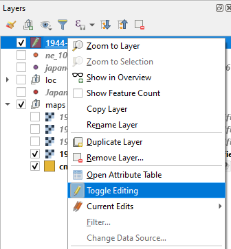
a, Right click on the shapefile in the QGIS layers window, select “Toggle Editing.”
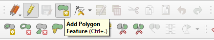
b. Navigate to the Digitization Toolbar, find and click the icon for “Add Polygon Feature”
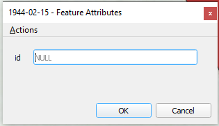
c. The mouse icon should transform into a crosshair. Now it is time to lay the first point by clicking on the image and repeat the process until the desire chuck has been highlighted in the a red polygon. When satisfied with the work right click to complete the feature. You will be immediately prompted with a “Feature Attributes” window. Click ok.

d. Congratulations…you’ve only just begun. Now would be a good time to save your progress. Again right click on the shapefile in the in the QGIS layers window and select “Save Layer Edits.” Do this often.

Now it is time to continue digitizing the portions in the South Pacific. From here you are going to make use of QGIS’ snapping tool. The snapping tool allows you to digitize, in part, by using the geometries of existing features. That is a fancy way of say “tracing without overlapping.”
e. Again click on “Add Polygon Feature.” Also click on the magnet icon on the snapping toolbar.

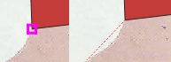
f. Hover the crosshair over the desired vertex and you’ll notice that it will be outlined with a pink box. Click on that box and then turn off the snapping tool. The digitization tool is now “anchored” and you can proceeded with digitizing the rest of the feature to include the edges of the image.
To complete the feature activate the Snapping tool, hover over the desired vertex, click the pink box, turn off the Snapping tool, and right click. You should again be prompted by the “Add Polygon Feature.” Click ok.
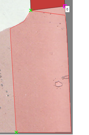
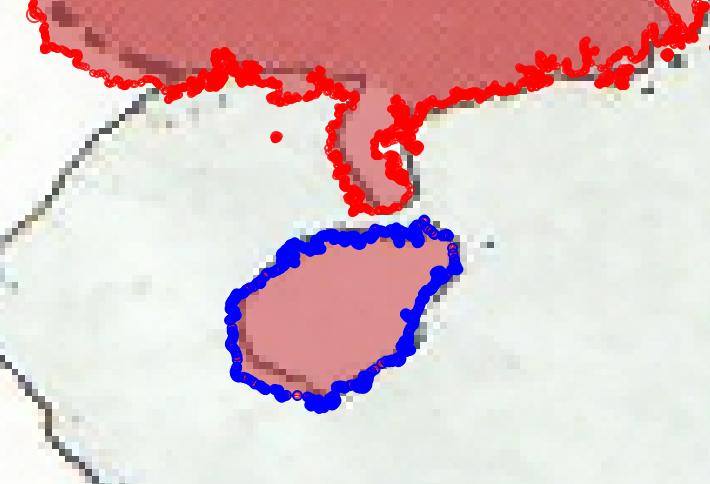
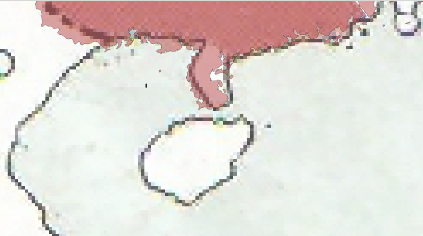
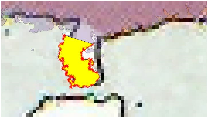
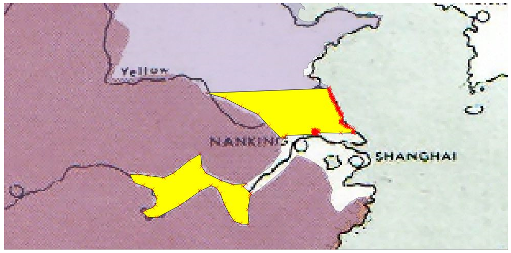
You may notice that there is a ring on the map which is not yet reflected in our digitization. The island hopping campaign conducted by the Allies left many such bypassed locations. You’ll need to reflect in our shapefile.
Thankfully, there is a solution!
g. Navigate to that portion of the map, it would be best to zoom in a little. Then navigate to the “Advanced digitization Toolbar” and select “Add Right.” The cursor should have once again transformed into a crosshair icon.

f. Trace around the bypassed area on the map with a sufficient number of points and right click when you are completed. You should have added a ring to the shapefile feature.
Now would be a good time to save the layer edits and the project.
g. Now it is time to fly solo…don’t worry I’ll be here when you get back! Repeat the processes outlined above to digitize the rest of the Allied advance in the South Pacific. You’ll want to stop somewhere south of Indian shoreline west of Rangoon, Burma.
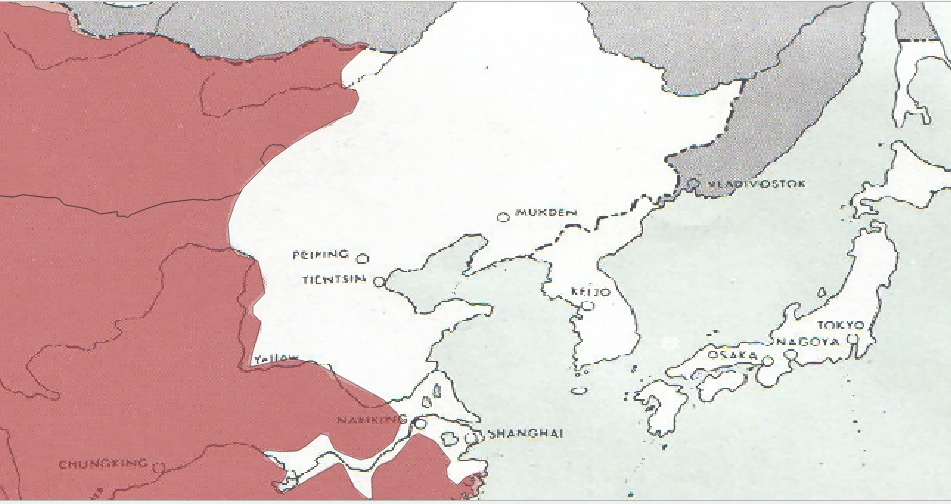
Step 4, The Not-So-Easy Part, part 1. Great you’re still here! Now examine rest of the map. You may noticed that the remaining portions of the map to be digitized are heavily aligned with China’s maritime boundary, its riverine boundary with Vichy Indochina and Mongolia’s northern boundary with the USSR. Rather than digitize these elements freehand we are going to “harvest” them from the existing boundary shapefile. For this I am going to use a shapefile of current political boundaries. Despite being anachronistic, the features we are drawing on, China’s coastline, the Mongolian-Russian Border, and the China-Vietnam border are largely the same as they were in 1944 and current boundary data is more accurate than is what is available in historic shapefiles.
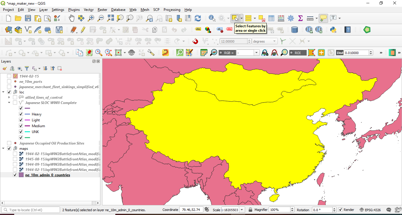
a. Highlight the base layer in the QGIS layers menu. Navigate to the “Attributes Toolbar” and select “Select Features by area or single click,” Click and drag so Mongolia and China are selected.
b. Right click on the base layer, select Export -> Save Features As
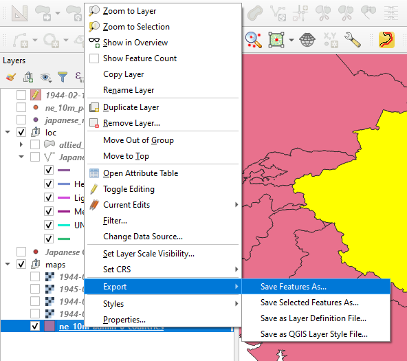
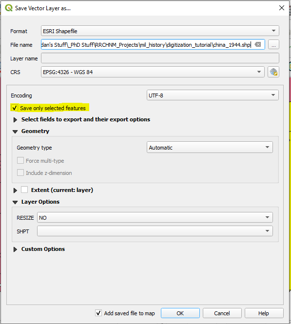
c. A window entitled “Save Vector Layer as…” should appear. Navigate to a desired file path using the “…” button and name the soon-to-be new shapefile. Ensure that “Save only selected features” and “Add saved file to map” are checked.
Hit ok.
d. You should now have a brand new China and Mongolia added to the map.
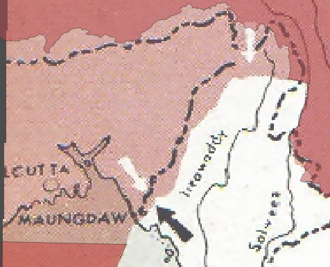
Step 5 The Not-So-Easy Part, China-India-Burma Theatre.
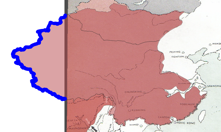
Our next step will be to digitize the portion between the South Pacific section you digitized manually earlier and our exported China shapefile. Zoom in on the China-India-Burma theatre portion of the map. Notice how the front deviates from the Chinese border? In order to recreate that, you’ll need to delete that portion from our new Mongolia-China shapefile.
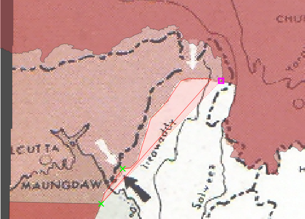
a. Zoom in to that portion of the map. Navigate to the Advanced Digitization Toolbar and select “Split Features”
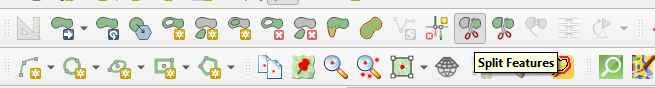
b. Click on a portion of the area of interest immediately outside the area to be deleted and then click along the front line and then right click on a portion immediately outside the area to be deleted. QGIS will split that portion off of our exported Mongolia-China shapefile.

c. How select the split portion and delete it.
d. Now you’re going to digitize the rest of the China-India-Burma theatre. Navigate to the digitization toolbar and select create new feature. Then navigate to the Snapping Toolbar turn on the “Enable Snapping” and “Enable Tracing”

e. As you did earlier start use the snapping tool to begin the new feature on the vertex of the South Pacific portion you digitized earlier. This time choose the eastern vertex. Turn off the snapping tool and digitize by hand the frontline between the existing shapefile and the exported Mongolia-China shapefile. Now, navigate back to the “Snapping Toolbar” and reactivate “Enable Snapping” and turn on “Enable Tracing.”
As before the snapping tool will allow you to align the new vertex with an existing one. Click on the pink box which will appear and trace the icon over the Chinese border. The Enable Tracing function will “hook” the cursor to this feature. Trace until the edge of the map, again click on the pink box which appears and trace down to the other side of the South Pacific shapefile that you created earlier. Click on the pink box which will appear and then right click. You should once again be prompted with the “Feature Attributes” window.
Click ok.
Take a deep breath.


Step 6, The Not-So-Easy Part, Southern and Eastern China.
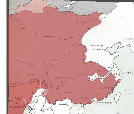
Now it is time to complete this odyssey by digitizing the portions of the map in China. Unlike the South Pacific section you will remove existing sections of our exported Mongolia-China shapefile.
a. Start with the island of Hainan and the neighboring peninsula. Activate the Vertex tool from the the “Digitization Toolbar.” Drag and select the vertices which compromise the island of Hainan and delete them.

b. Use “Split Features” to remove the Leizhou Peninsula.
c. Repeat the process for the area around Canton/Hong Kong

c. Repeat splitting process for the areas around Nanking, Shanghai and Yangtze river.
d. Now it is time to remove the expanse of Japanese occupied Eastern China. As with your earlier efforts this will best preformed in chunks.
e. Delete the vertices which extend beyond the bounds of our map.
Note you may have to clean up small portions with the Vertices tool. You may also need to use the “Check Validity” tool to clean up any errors which you may encounter and prevent you from proceeding.
Step 7, The Not-So-Easy Part…the Dissolve.
Almost there…I promise. Now you’ll need to dissolve the individual features within the original shapefile which covers the South Pacific and the China-India-Burma theatre and merge that with the exported Mongolia-China shapefile.
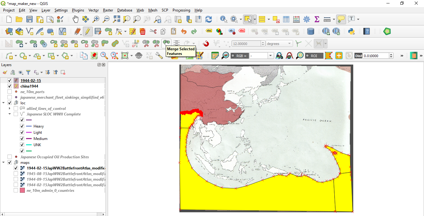
a. Select the created shapefile from the Layers menu. Select all four portions of the shapefile. Navigate to the Advanced Digitization Toolbar and select “Merge Selected Feature.” A window titled “Merge Feature Attributes” will appear.
Click ok.

b. Repeat the same process for the exported China shapefile.
Step 8, The Not-So-Easy Part…the Merge.
Now it is time to merge the shapefile that you created with the exported Mongolia-China shapefile. First you are going to delete a bunch of superfluous metadata from the exported Mongolia-China shapefile. This is modern data it will only clutter up our final product.
a. Navigate to the Mongolia-China shapefile in the Layers menu. Right click, select properties and navigate to fields.
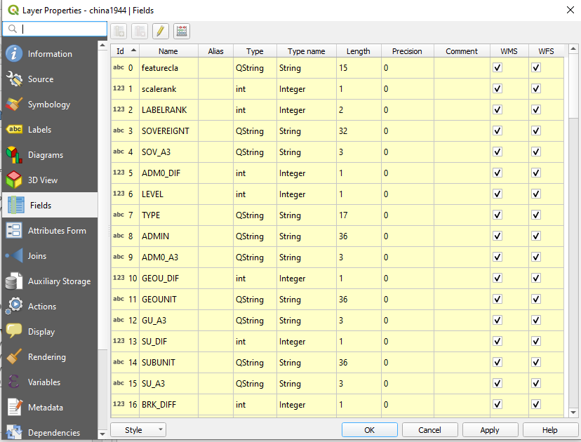
b. Ensure that editing mode is on by clicking the pencil icon. Highlight all the columns and hit “Delete Fields.” Go ahead and save your layer edits.
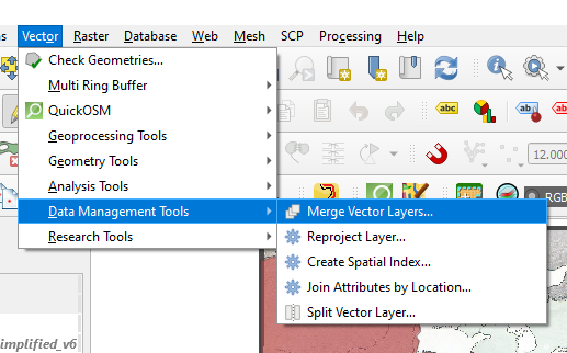
c. Navigate to Vector -> Data Management Tools -> Merge Vector Layers
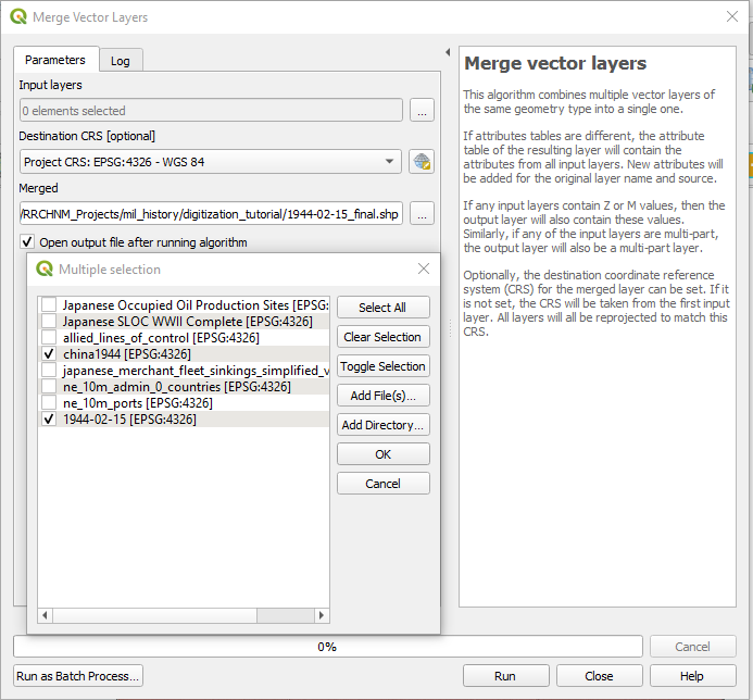
d. The Merge Vector Layers window will appear. Set the Project CRS to ESPGL 4326 – WGS 84. Choose an output file by clicking the “…” icon by the “Merged” panel. Select the shapefiles by clicking the “…” icon by the Input layers panel. Select the export China-Mongolia shapefile and the one that you created from scratch.
Hit ok.
Let the science happen.
e. Step 9, The Not-So-Easy Part…Clean up.
Second to last step I swear! While our two shapefiles are now combined the new shapefile will likely contain multiple superfluous features. Most of these are likely an assortment of random islands and inlets which were not swept up and deleted during the earlier processes.
a. Navigate to the new shapefile in the layers panel and toggling editing. As before, select both features, navigate to the Advanced Digitization Toolbar and “Merge Selected Features.”
b. Navigate to the new and newly merged shapefile. Select the feature from the main window.

c. Right click on the shapefile in the layer window. Select “Open Attribute Table.” And select “Invert Selection”

d. This will select the random geometries which were not swept up during your earlier work.
e. Hit “Delete selected features.”

f. Navigate to the layer properties menu as you did before and delete the existing fields.
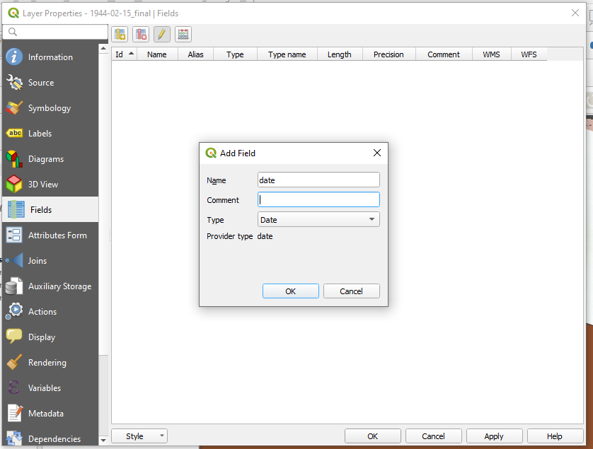
g. Add a new field by clicking the “Add Field Icon. The Add Field window will appear. Name it “date” and select Date from the type dropdown menu.
Hit ok.
And then hit ok to close the Layer Properties Menu
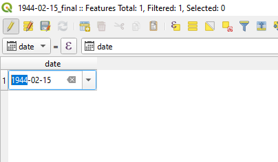
h. Open the attributes layer for the new shapefile. And enter a date into the field, 1944-02-15. Save your layer edits, toggle editing, and save your project.
And with that, you’re done!

Stay tuned to for Rebuilding a War, Part 2: Map Georectification and Feature Digitization, Lines!